Xavier and He Initialization
Xavier and He initialization, the fixes that keep signal variance stable as a network gets deeper.
Two standard recipes, one of them fatal
Xavier initialisation, applied correctly, to a ReLU network. Eight layers.
Both of those are the standard, correct, widely recommended initialisation. One of them threw away 94% of the training signal before it reached the first layer, and the only difference between them is a factor of two.
Before this page - 2 pages, both immediately relevant2
No forward dependencies. This is the one page in this group that is fully self-contained against the reading order.
Set n to 100 and click through all three schemes without touching anything else. Watch the std readout and the flat-zone percentage, not the bars.
 0:14
0:14What this animation shows
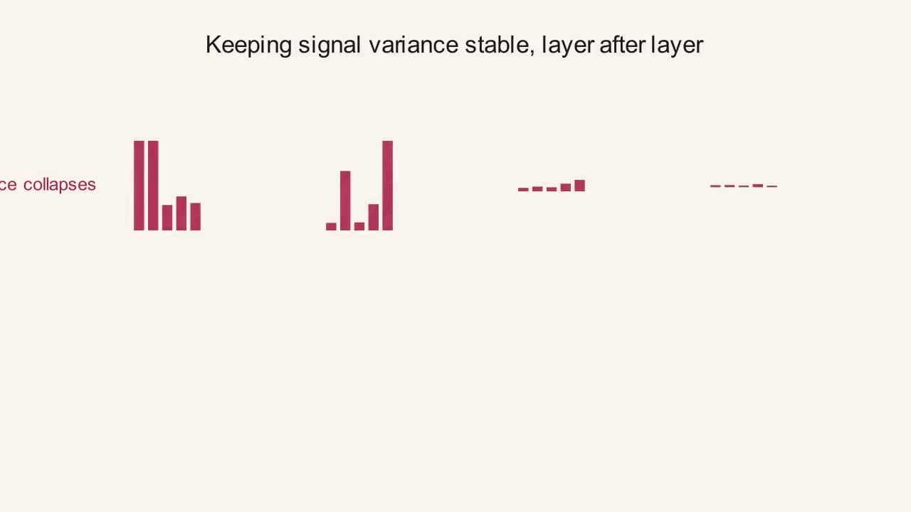
Two rows of small per-layer histograms build up across four layers. The top row, labeled "naive init," visibly collapses - each layer's spread of values shrinks toward nothing by layer four. The bottom row, labeled "Xavier / He," keeps a consistent spread across all four layers, showing exactly what these initialization schemes fix: keeping signal variance stable as a network gets deeper.
Each bar is the share of 1,000sampled neurons whose pre-activation value landed in that range. The shaded bands mark roughly where sigmoid/tanh go flat (|x| > 3) - gradient close to zero there, before training even starts.
Naive stays a fixed width no matter how wide n gets. Xavier and He rescale the draw so the spread stays roughly stable as n grows.
He initialisation uses exactly twice Xavier’s variance on a square layer. What is the 2 cancelling?
- aThe two directions, forward and backward
- bThe two in Var(output) = n·σ²
- cReLU throwing away half its input
- dNothing - it was tuned empirically
Commit to a guess, then open this
ReLU throwing away half its input. If the values arriving are symmetric around zero, ReLU zeroes half of them, which halves the average squared size of what comes out. So a ReLU layer has two multiplications, not one: n·Var(W) from the weighted sum, then ×0.5 from ReLU. He’s 2 exists to make 0.5 × 2 = 1. Take the 2 away and every layer halves the signal - which is LeCun initialisation on ReLU, and it is the top row of the block in rung 2, losing half the signal per layer and 0.00000095 of it over twenty.
The previous page showed the problem: a fixed-scale random weight draw makes a neuron’s typical output size depend entirely on how many inputs it has, growing or shrinking uncontrollably as networks get wider or deeper. Xavier and He initialization are the two standard fixes, each tuned for a different activation family.
Two words appear in every formula below, so here they are in plain language. A layer’s fan-in is how many numbers arrive at each of its neurons, and its fan-out is how many neurons in the next layer each of its outputs is sent to. A layer taking 784 pixels and producing 256 hidden values has fan-in 784 and fan-out 256. Fan-in controls what happens to a signal moving forward, because it is the number of terms being added up. Fan-out controls what happens to a gradient moving backward, because it is the number of places a neuron’s error signal arrives from. Every initialisation scheme on this page is some choice about which of those two numbers to size the weights against.
Xavier (Glorot) initialization picks the variance of the random weights so that, on average, a layer’s output variance matches its input variance, keeping signal magnitude stable as it flows forward through the network, while also trying to keep gradient variance stable flowing backward. Those two goals want slightly different formulas, so Xavier splits the difference by averaging a layer’s fan-in and fan-out.
He (Kaiming) initialization exists because Xavier’s derivation implicitly assumes a roughly linear, zero-centered activation, true near x=0 for tanh and sigmoid. ReLU breaks that assumption outright: it zeros out exactly half its inputs on average, cutting the forward-pass variance in half at every single layer. He compensates by doubling the variance Xavier would use, exactly offsetting ReLU’s own variance-halving.
The mixing desk again, but this time the setting
The previous page was the problem: get any stage’s gain wrong and the chain clips or hisses. This page is the manual. Unity gain on a stage that sums n inputs is not 1 on the fader, it is 1/√n, because summing n independent signals raises the level by √n. And if the stage has a limiter after it that kills every negative half-cycle - which is what ReLU is - you have to push the fader up by √2 to compensate for what the limiter removes. That is He, exactly.
Where it breaks downA desk’s stages are independent. A network’s are not: layer 3’s ideal gain depends on what layers 1 and 2 actually did to the signal, which is why this only holds at step zero.
WordsTwo recipes and the one number they aim atWhat each scheme is for, and the number they are both trying to hit.Rung 01
A layer’s fan-in is how many numbers arrive at each of its neurons; its fan-out is how many neurons in the next layer each of its outputs is sent to. Fan-in controls the forward pass, fan-out the backward one, and every scheme here is a choice about which to size against.
Xavier picks the weight variance so a layer’s output variance matches its input variance, forward and backward. Those two goals want slightly different formulas, so Xavier averages fan-in and fan-out - which is why the formula has a sum in it, and why it hits its target exactly only on a square layer.
He exists because ReLU zeros half its inputs, halving the forward variance at every layer. He doubles Xavier’s variance to cancel exactly that halving, and sizes on fan-in alone.
Rule of thumb: sigmoid/tanh hidden layers → Xavier; ReLU-family hidden layers → He.
NumbersFive layers, three schemes, twiceThe claim that these keep the signal stable, checked over five layers, three ways.Rung 02
Compare this site’s actual current fixed-scale init: uniform(−1,1) has std=√(1/3)=0.5774 too - for THIS specific layer size, they happen to match exactly (n_in+n_out=6 is the one case where they coincide). A layer with n_in=100 instead would get Xavier std=√(2/102)=0.140028, over 4× smaller than this site’s current fixed 0.5774, which is exactly the shrink needed to counteract the variance-growth problem from the previous page.
The point of that variance is what it does over depth. Take a stack of five layers, each 100 wide, so n_in = n_out = 100 and Xavier’s Var(W) = 2/200 = 0.01. Each layer multiplies the incoming variance by n_in · Var(W):
The factor being exactly 1.0 is the entire design goal, stated as a number. Whatever variance goes in comes out unchanged, so depth costs nothing, and the hundredth layer sees values the same size as the first.
There is one honest caveat, and it is the reason the averaged form exists. That factor is exactly 1 only when n_in equals n_out. On a layer that changes width, say n_in=100 and n_out=25, Xavier gives Var(W) = 2/125 = 0.016 and the forward factor becomes 100 × 0.016 = 1.6:
That is the compromise the averaging buys. Sizing purely on n_in would hold the forward pass perfectly still and let the backward pass drift; sizing purely on n_out would do the reverse. Xavier splits the difference, so both directions drift a little rather than one drifting a lot. On networks whose layer widths change gradually, which is most of them, the drift is small enough not to matter.
He’s claim is the sharper of the two, so it is the more worth checking. Two things to settle first. The quantity being tracked below is the second moment, written E[a²], and it is not quite the variance from the previous page. E[…] means “the average value of, if you repeated this over and over”, so E[a²] is the average of the squared activations, with no subtraction of the mean. The two agree whenever the values are centred on zero, and they part company when they are not: ReLU’s output is never negative, so its average is above zero and the two genuinely differ. He et al. track the second moment for exactly this reason. Second, the halving assumes the values arriving at ReLU are symmetric around zero, which is true at initialisation with zero biases and stops being exactly true once training has moved the biases.
The 2 in 2/n_in is doing one job and it is visible in the middle row: it cancels the 0.5 that ReLU introduces, 0.5 × 2 = 1, and the product comes out at exactly 1. Take the 2 away and every layer halves the signal, which is the top row. That is the whole of He initialisation.
The scheme is designed for the first forward pass; after that, other machinery, including batch normalization, takes over the job of keeping activations well-scaled.
PictureOne layer in the histogram, eight layers in the bar chartThe one-layer picture and the eight-layer picture, and why you need both.Rung 03
At n = 100 in Figure 02, naive reports std 5.773 and 62.2% of the layer in the flat zone; Xavier reports std 1.018 and 0.2%; He reports std 1.382 and 3.3%. He is deliberately wider than Xavier - √2 wider - because it is compensating for a halving that this histogram cannot show, since the histogram plots pre-activations and the halving happens after.
That halving is what the second instrument makes visible. Set it to ReLU, depth 8, weight scale 1.0 and the readout says the per-layer factor is 1.0000 and the gradient after eight layers is 1.000e+0 - He’s design goal, drawn as eight bars of identical height. Now drag the weight scale to 0.7, which is √0.5 to the nearest step the slider allows, and which is what Xavier’s variance gives a square ReLU layer: the factor is 0.7000 and after eight layers 5.76e-2. Same network, same activation, same depth. The only change is a factor of √2 in the initialisation, and 94% of the gradient is gone.
This axis is log-scaled and centered on 1.0 - each gridline above center is a ×10 growth, each gridline below is a ×10 drop, because the real values shrink or grow so fast that on an ordinary axis every bar past the second one would look like it's touching zero or flying off the top.
At weight scale ≈1×, each layer's factor sits right at the tipping point between the two regimes - nudge the slider either direction to see which way it goes.
EquationBoth formulas, and where the 6 comes fromFour formulas, and the substitution that turns one into the other.Rung 04
The √(6/(n_in+n_out)) bound looks arbitrary and is not. A uniform distribution over (−a, a) has variance a²/3, which is the fact the previous page used to get 1/3 out of uniform(−1, 1). Set that equal to the variance you wanted and solve:
The 6 is a 2 and a 3 that were multiplied together on the way past. Every “why is there a 6 in this formula” in deep learning initialisation is this same substitution.
General caseAny layer shape, and what this looks like in codeThe general formula at real layer sizes, then the one parameter frameworks actually ask you for.Rung 05
Comparing the two on one specific layer shape understates the relationship. On any layer where n_in = n_out, Xavier’s variance is 2/2n = 1/n and He’s is 2/n, so He is always exactly twice the variance and √2 = 1.414 times the standard deviation. Here is what that looks like at sizes you would actually build:
The first row is the small layer from the worked examples above; the 784 → 256 row is the first layer of a network reading 28×28 pixel images, which is where most people meet these numbers for the first time.
Frameworks do not usually ask you for a variance. They ask for a gain, a multiplier applied on top of a base scale, chosen to suit the activation function that follows the layer. The base is 1/n_in, and:
So kaiming_normal_ and xavier_uniform_ are not two unrelated functions, they are the same variance calculation with a different denominator and a different gain. The tanh gain of 5/3 is a refinement on plain Xavier: tanh compresses its input slightly even near zero, so a little extra variance going in keeps the variance coming out closer to 1.
Flagged as simplified: every calculation on this page assumes the weights are independent of each other and of the inputs, and that the inputs are zero-centred. Both hold at initialisation, which is the only moment these schemes are asked to do anything, and neither holds after training begins.
Why this and not that
Why does Xavier average fan-in and fan-out rather than picking one?
Because the two directions want different answers and you only get one draw. Sizing on fan-in holds the forward pass perfectly still and lets gradients drift; sizing on fan-out does the reverse. Averaging makes both drift a little instead of one drifting a lot. The narrowing-layer block in rung 2 is what that compromise costs: 1.6× per layer on a 100 → 25 layer, rather than 1.0×.
Why does He use fan-in only, then?
He et al. showed the forward and backward variance conditions for ReLU differ by exactly the ratio n_out/n_in, and that either choice keeps the whole product over all layers bounded, so the compromise buys less than it does for Xavier. Fan-in is the one they recommend, and it is what kaiming_normal_ defaults to.
Does the ReLU halving argument hold once training starts?
No, and rung 2 says so before it uses it. The halving assumes the values arriving are symmetric around zero, which is true at initialisation with zero biases and stops being exactly true the moment the biases move. Initialisation only has to be right once, at step zero, which is the only moment it is asked to do anything.
Why track the second moment E[a²] rather than the variance?
Because ReLU’s output is never negative, so its mean is above zero and the two quantities genuinely differ. For a zero-centred signal they are the same number and the distinction is free; after a ReLU it is not, and He et al. track the second moment for exactly that reason.
If batch normalization rescales every layer anyway, does initialisation still matter?
Less, and not zero. Batch norm takes over the job of keeping activations well-scaled from about step one, but the first forward pass and the first backward pass happen before it has any statistics, and a network that produces inf on its first forward pass never gets to step one. Rung 2 makes this explicit.
- Xavier
- Xavier Glorot’s first name. The paper is Glorot & Bengio 2010, which is why the identical scheme is called “Glorot initialisation” in Keras and “Xavier” in PyTorch. Two names, one person, one formula.
- He
- Kaiming He’s surname, and it is pronounced closer to “huh” than to the English word. Hence kaiming_normal_ in PyTorch and “He initialisation” in papers: same person, named the other way round from Xavier, which is exactly why both naming conventions look arbitrary.
- LeCun init
- Yann LeCun, from the 1998 Efficient BackProp chapter. It is the ancestor of both: 1/n_in, no activation correction at all.
- Gain
- Straight from amplifier engineering, where gain is how much a stage multiplies its input. In torch.nn.init.calculate_gain it means precisely that, and the ReLU gain of √2 is the same 2 as He’s.
- Fan-in
- See the previous page; from digital logic, and it means the same thing here.
- What is happening
Xavier’s variance on a square ReLU layer gives a per-layer factor of
√0.5 = 0.7071, and 0.7 is the nearest the slider reaches. Eight layers of that is 0.0576, so 94% of the gradient is gone before it reaches layer 1. Nothing crashes and no number isNaN; the network simply learns its early layers about seventeen times slower than its late ones.- Fix
kaiming_normal_(w, nonlinearity='relu'), which isVar(W) = 2/n_in. Compare against He by setting the weight scale to 1.0.- Watch for
- Eight bars stepping visibly downward on the log axis, and the readout’s ‘vanishing’ verdict. Then set the scale to 1.0: eight bars of identical height and 1.000e+0.
- What is happening
Identical weight scale, identical depth, opposite failures. With tanh the per-layer factor is 0.588 and the gradient vanishes to 1.4% of what arrived (1.43e-2 over eight layers). With ReLU at the same 1.4 the factor is 1.400 and the gradient explodes to 1.476e+1, fifteen times what arrived. The activation function is half of the per-layer factor, and an initialisation chosen without reference to it is a coin flip about which direction the network fails in.
- Fix
Xavier for sigmoid and tanh, He for the ReLU family. The rule of thumb in rung 1 is this mistake, written as advice.
- Watch for
- The same slider value producing a ‘vanishing’ verdict on one activation and an ‘exploding’ verdict on the other, one dropdown click apart.
- What is happening
The gradient after eight layers is now 6,561 times what arrived at the output. The compounding that was destroying the signal is the identical mechanism that is now destroying the weights; only the direction changed. There is exactly one factor value that does neither, and it is 1.
- Fix
Do not tune the scale by feel. Compute it:
2/n_infor ReLU,2/(n_in + n_out)for tanh. If the gradient is still vanishing at the right scale, the answer is a residual connection or a normalization layer, not a larger number.- Watch for
- The bars flipping colour and growing upward off the top gridline, and the verdict switching to ‘exploding’.
- What is happening
This is a perfect result and it is a result about step zero. He initialisation sizes the initial draw so the factor starts at 1; nothing holds it there. Training moves every weight, and by epoch ten the factor is whatever training made it. The eight identical bars are a photograph of the first forward pass, not a guarantee.
- Fix
Initialisation buys you a healthy start. Keeping it healthy is batch normalization, residual connections and gradient clipping, which are the next two pages and the convolutional networks module.
- Watch for
- Eight bars at exactly the same height - the only configuration in this widget that does that - and the word ‘stable’ in the readout.
- What is happening
Both Xavier readings look perfect, and both are, because this widget assumes a square layer where fan-in equals fan-out: n = 100 gives std 1.018 and 0.2% flat, n = 200 gives std 1.004 and 0.3% flat. Real layers change width, and Xavier’s average then splits the difference rather than hitting 1 exactly: on a 100 → 25 layer the forward factor is
100 × 2/125 = 1.6, so the variance grows 1.6× per layer and reaches 10.4858 by layer five - the block in rung 2. The histogram cannot show this, which is precisely why the block exists.- Fix
On layers that change width sharply, size on fan-in for the forward pass, and know that you have chosen a direction. On networks whose widths change gradually, which is most of them, the drift is small enough not to matter.
- Watch for
- Two flawless readings from a widget that is answering an easier question than your network asks.
This axis is log-scaled and centered on 1.0 - each gridline above center is a ×10 growth, each gridline below is a ×10 drop, because the real values shrink or grow so fast that on an ordinary axis every bar past the second one would look like it's touching zero or flying off the top.
At weight scale ≈1×, each layer's factor sits right at the tipping point between the two regimes - nudge the slider either direction to see which way it goes.
Each bar is the share of 1,000sampled neurons whose pre-activation value landed in that range. The shaded bands mark roughly where sigmoid/tanh go flat (|x| > 3) - gradient close to zero there, before training even starts.
Naive stays a fixed width no matter how wide n gets. Xavier and He rescale the draw so the spread stays roughly stable as n grows.
- 01Find the weight scale at which a ReLU network of depth 8 neither vanishes nor explodes, and say what initialisation it corresponds to.
Hint
Read the per-layer factor line, not the bars.
Answer
Weight scale 1.0, giving a per-layer factor of exactly 1.0000 and a gradient of 1.000e+0 after eight layers. For a square ReLU layer that corresponds to
Var(W) = 2/n, which is He initialisation. Every other slider position on this widget either loses or gains signal at every layer, compounding. - 02Compute Xavier’s and He’s standard deviation for a 784 → 256 layer, then find the histogram setting that comes closest.
Hint
Xavier is
√(2/(n_in+n_out)), He is√(2/n_in). The histogram only has onenslider and it stops at 200.Answer
Xavier:
√(2/1040) = 0.043853. He:√(2/784) = 0.050508. Both are in the six-row table in rung 5. The histogram cannot reach n = 784 - its slider stops at 200 - and that limit is worth noticing: at n = 200 the naive scheme is already at std 8.502 with 72.4% of the layer dead, and a real first layer is nearly four times wider than that. The widget runs out of slider before this initialisation runs out of ways to fail. - 03Show that He is exactly √2 times Xavier on a square layer, using the widget’s own readouts.
Hint
Compare the std at the same n for the two schemes.
Answer
At n = 100 the widget reports Xavier std 1.018 and He std 1.382, a ratio of 1.358 against the theoretical
√2 = 1.414; at n = 200 it reports 1.004 and 1.427, ratio 1.421. The wobble is sampling noise over a thousand draws, not a real disagreement - the analytic values are exactly 1.000 and 1.414. The relationship is exact and the widget is measuring it, which is a useful thing to have seen once. - 04Make tanh explode.
Hint
tanh’s slope at the widget’s pre-activation of 1.0 is 0.41997. What does the weight scale have to beat?
Answer
Weight scale 2.5 gives a factor of 1.0499, the first slider position above 1.0, and after eight layers 1.477. At 3.0 the factor is 1.2599 and eight layers give 6.350. Now try the same with sigmoid: it cannot be done. Sigmoid’s slope at 1.0 is 0.19661, so the weight scale would have to exceed 5.09 and the slider stops at 3.0. Sigmoid is not merely worse than tanh here, it is worse by a factor that puts exploding gradients out of reach and vanishing ones out of avoidance.
- 05Using the rung 2 blocks, work out how many layers LeCun initialisation can survive on a ReLU network before losing 99% of the signal, then check the arithmetic against the widget.
Hint
LeCun’s per-layer factor on ReLU is 0.5. When is
0.5^k < 0.01?Answer
0.5⁷ = 0.0078, so seven layers. The block in rung 2 gives the first five (1.0 → 0.5 → 0.25 → 0.125 → 0.0625 → 0.0313) and0.5²⁰ = 0.00000095for twenty. The widget cannot set a factor of exactly 0.5 for ReLU - its slider steps at 0.1 - but 0.5 on ReLU is the closest, and at depth 7 it reports 7.81e-3. Seven layers is not deep. This is why the 2 in2/n_inexists and why it is the entire content of the He paper.
- torchvision ResNetIts weight init is one line -
kaiming_normal_onm.weight, withmode='fan_out'andnonlinearity='relu'- applied to every conv layer in the model. That line is this page. - He et al., 2015The paper reports that a 30-layer plain ReLU network initialised with Xavier failed to train at all, while the same network with He’s variance converged. The gap between the two is the factor of 2 in rung 4.
Every layer is a photocopier. Set the zoom to exactly 100% or by page five you have either a dot or a blur.
Xavier and He are two ways of computing 100% - and the only difference between them is that ReLU throws half the page away.
These two schemes solve one problem completely: the network starts healthy. They say nothing at all about what happens after that. A network can be perfectly initialised, train smoothly, drive its training loss to almost zero, and be useless - because it has learned the exact noise in the examples it was shown rather than the pattern behind them. Nothing on these two pages can detect that, because it is not a numerical failure. Every number stays in range and every gradient stays healthy while it happens.