Training-Time Regularization
Training-procedure techniques - dropout, early stopping, batch normalization, and data augmentation - that fight overfitting without changing the loss formula.
94% in training, 71% one flag later
A network that scores 94% during training and 71% the moment you switch it to evaluation mode. Same weights, same data, one flag.
Both rows are correct. Both are what the layer is supposed to produce in its own mode. And the layer downstream of them has been calibrated against numbers it will never see again.
Before this page - 3 pages needed, 1 borrowed from the next page4
Regularization
the previous page; this page is explicitly the other half of it, procedure regularizers rather than loss-formula ones, and it reuses overfitting, bias and variance without redefining themWeight Initialization
batch normalization is an argument about the mean and the variance of a layer’s inputs, and variance is defined thereGradients and Gradient Descent
early stopping is a rule about when to stop taking steps, and the gamma/beta block is an ordinary gradient updateBackpropagation
“the gradient arriving at y” appears in the gamma/beta block one page early. It means: if this output number changed a little, how much would the loss change. The values are simply given here; the procedure that produces them is the next page.comes later
Press ‘Resample mask’ five or six times and watch the four numbers change. Then switch to Inference and press it again - nothing happens, and that is the point.
 0:14
0:14What this animation shows
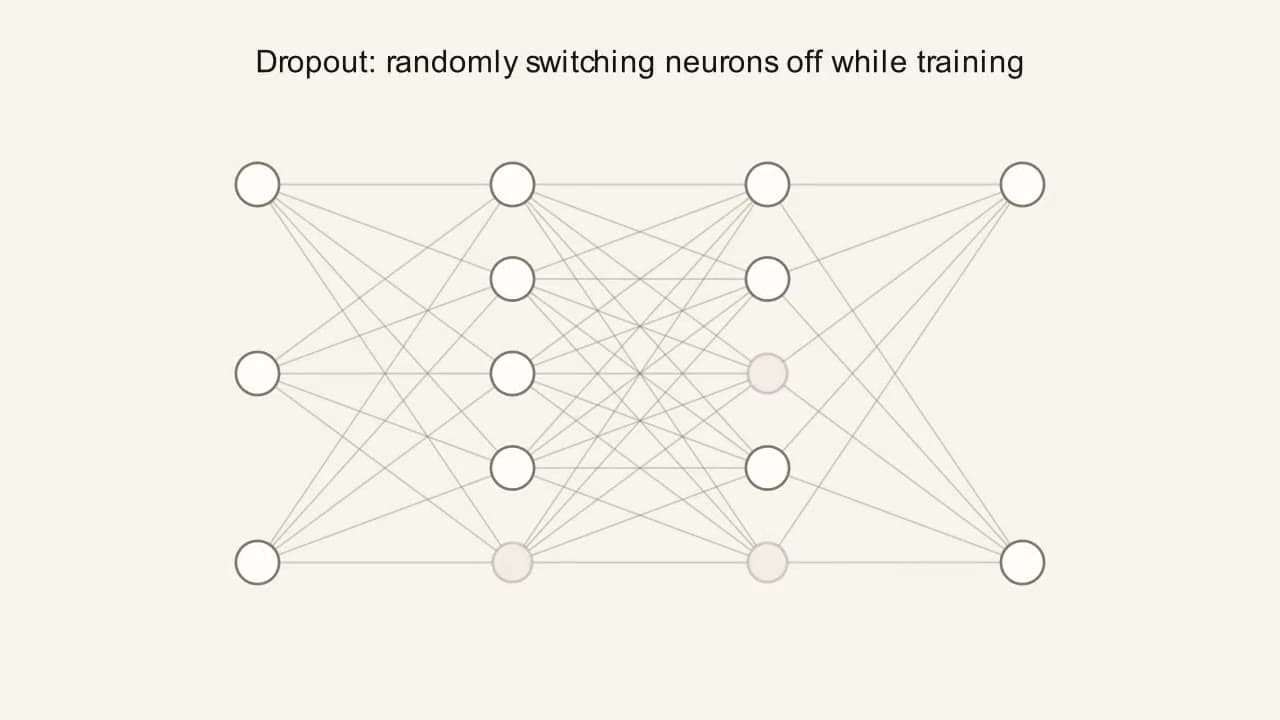
A small multi-layer network lights up, and then, over a few rounds, random hidden neurons fade out and shrink ("dropped") before fading back in, repeating with a different random set each round. At the end, every neuron lights up together with the caption "at test time, every neuron is back on." This is dropout: randomly disabling neurons during training so the network can't over-rely on any one of them.
Greyed, dashed neurons were dropped this draw. Survivors get scaled up by 1/(1−p) so the layer's expected total signal stays the same.
Dropout at p = 0.5 switches off half a layer’s neurons. What does it do to the survivors?
- aNothing - the rest carry on as normal
- bHalves them, so the total stays the same
- cDoubles them, so the total stays the same
- dAdds noise to them
Commit to a guess, then open this
Doubles them. The surviving activations are divided by (1 − p) = 0.5, so 0.8 becomes 1.6 and 1.2 becomes 2.4 - which is what the widget’s readout shows. The reason is that the next layer has to see roughly the same total signal whether or not units were dropped, because at prediction time nothing will be dropped at all. Averaged over all sixteen possible masks the layer’s output comes back to exactly [0.8, −0.3, 1.2, 0.5], unchanged. Unbiased on average, and different on every single pass - and that difference is the regularizer.
The previous page covered regularizers that change the loss formula itself. This page covers a different category: techniques applied to the training procedure or the network’s structure, rather than to the loss.
Dropout. During training, randomly and independently switch off a fraction of neurons on every forward pass, as if training a huge ensemble of thinner sub-networks that all share weights. No single neuron can be relied upon to always be present, so the network is forced to spread information across multiple redundant paths instead of a few neurons over-specializing together. At test time, use the WHOLE network, but since training only ever saw a thinned-out version, surviving activations get scaled up during training so the expected total signal stays the same (“inverted dropout”).
A trap worth stepping around before the numbers. There are two conventions for what the letter p means in dropout, and they are inverses of each other. This page uses p = the probability a unit is dropped, which is PyTorch’s convention and TensorFlow’s current one: nn.Dropout(0.5) drops half the units. Some sources, including the CS231n course notes, use p = the probability a unit is kept, and their scaling factor is therefore 1/p where this page’s is 1/(1−p). Both describe identical behaviour.
Batch normalization. As a network trains, the distribution of values flowing into any given layer keeps shifting, because every earlier layer’s weights are also changing, a moving target that makes each layer’s job harder. Batch Normalization forces every layer’s inputs to have a fixed mean (0) and spread (1) within each mini-batch, then hands back two learnable knobs, a scale and a shift, so the network can undo that forcing if it turns out to need a different mean or spread for that particular layer.
Early stopping depends entirely on having a validation set. Split your data into three parts before training. The training set is what the network learns from and what the loss is computed on. The validation set is held out, never trained on, and scored periodically to see how the network does on data it has not memorised; it is what you use to make decisions, like when to stop or which λ to pick. The test set is held out from that too, scored once at the very end, and never used to make any decision at all, because every decision you make using a set is a way of slowly fitting to it. A typical split is 80/10/10.
That is what makes early stopping possible. Training loss cannot tell you when to stop, because it falls essentially forever; a network that has memorised the training set has a beautiful training loss. Validation loss is measured on data the network has never adjusted itself to fit, so when it starts rising, the network has stopped learning the pattern and started learning the sample.
Training with players missing
A football side that always practises eleven-a-side builds moves that depend on one particular winger being in one particular place. Practise with three players pulled out at random every session and nobody can be relied on, so everyone learns to cover. That is dropout, and the ensemble claim is literal: with four players there are sixteen possible line-ups and training visits them at random. The catch is that on match day you field the whole eleven, a team that never actually trained together, which is exactly why the survivors get scaled up during training.
Where it breaks downFootballers know who is missing. A neuron has no idea; it just receives a smaller number and gets no gradient at all.
WordsFour techniques, none of which touch the lossWhat each technique does, and the one vocabulary trap that will otherwise cost you an afternoon.Rung 01
The previous page covered regularizers that change the loss formula itself. These four are applied to the training procedure or the network’s structure instead.
Dropout switches off a fraction of neurons at random on every forward pass, as if training a huge ensemble of thinner sub-networks that all share weights. No single neuron can be relied on, so the network spreads information across redundant paths. At test time the whole network is used, so survivors are scaled up during training to keep the expected total signal the same.
The p trap: this page uses p = probability of being dropped, which is PyTorch’s convention. CS231n and others use p = probability of being kept, with 1/p scaling rather than 1/(1−p). Identical behaviour, opposite letters.
Batch normalization forces every layer’s inputs to a fixed mean of 0 and spread of 1 within each mini-batch, then hands back a scale and a shift so the network can undo it where it needs to.
Early stopping needs a validation set: training data to learn from, validation data to make decisions with, test data scored once at the end and never used to decide anything. A typical split is 80/10/10. Training loss cannot tell you when to stop because it falls essentially forever; validation loss can, because the network never adjusted itself to fit it.
One mechanism used below and worth naming now: a running average blends each new measurement into a stored value instead of replacing it - keep 90% of what you had, add 10% of what you just saw. You do it this way because any single mini-batch’s mean and variance are noisy, and inference needs one fixed pair of numbers rather than whichever batch happened to arrive last.
NumbersEvery technique, workedDropout twice over, the patience counter traced, and batch norm in both of its two modes.Rung 02
Dropout. p=0.5, layer activations h=[0.8, −0.3, 1.2, 0.5], and this particular random draw happens to keep units 1 and 3:
One random draw does not show an ensemble. Here are two draws over the same layer, plus the average over every possible draw:
Unbiased on average is not the same as unchanged. Each individual forward pass is noisy, and the scaling makes that noise larger, not smaller. For a unit with activation h, the variance introduced is h²·p/(1−p):
That noise is the regularizer. It is also why p = 0.8 is rarely a good idea: past a point, the layer’s output is more noise than signal. Common values are 0.5 for fully connected hidden layers and 0.1 to 0.2 for convolutional ones, which have far fewer parameters per unit and need less help.
The backward pass needs no special rule, which is worth seeing rather than being told. The mask is just a multiplication by a constant, so the gradient gets multiplied by the same constant on the way back:
A unit that was dropped receives exactly zero gradient, so its incoming weights are not updated on that pass at all. That is the second half of dropout’s regularizing effect: not only does the network have to work without any given unit, no unit gets to learn from every example.
That is dropout in full. Next, a technique that regularizes not by changing what a layer computes but by changing when training stops.
Early stopping. Track validation loss per epoch, stop when it hasn’t improved for some number of consecutive epochs (“patience”), and keep the weights from the BEST epoch, not the last one.
| Epoch | Train loss | Validation loss |
|---|---|---|
| 1 | 0.90 | 0.95 |
| 2 | 0.74 | 0.68 |
| 3 | 0.61 | 0.48 |
| 4 | 0.52 | 0.39 |
| 5 | 0.45 | 0.34 |
| 6← keep this one | 0.40 | 0.30 |
| 7 | 0.36 | 0.33 |
| 8 | 0.34 | 0.38 |
| 9 | 0.32 | 0.41 |
| 10 | 0.31 | 0.44 |
Train loss falls steadily through all 10 epochs. Validation loss bottoms out at epoch 6 (0.30), then climbs for the rest of training. With patience = 3, here is exactly when the stop fires and which weights survive:
Two things that trip people up. Patience exists because validation loss is noisy: a single bad epoch is not evidence of overfitting, and a patience of 1 would stop most runs far too early. And the epochs after the best one are not wasted; you had to run them to find out that epoch 6 was the best. Early stopping always costs you patience epochs of hindsight.
That is the second technique in full. The third, batch normalization, is the longest block here - it has more moving parts, so take it in stages: first what it computes, then why the tiny constant in its formula matters, then how its two learned knobs actually get updated.
Batch normalization. Mini-batch of 4 pre-activation values x=[2.0, 4.0, 4.0, 6.0]:
Before the next block, what ε is doing in that denominator. It is a tiny constant, usually 1e-5, added to the variance purely so the division cannot blow up. If every value in a mini-batch happens to be identical, the variance is exactly 0, and without ε you would divide by zero. With ε you divide by √0.00001 = 0.003162 instead and every normalized value comes out as 0, which is the sensible answer: values that were all identical carry no information to spread out.
ε is invisible in normal operation and decisive in the one case that would otherwise crash. That is what a numerical-stability constant is for. The demo in rung 3 uses the same ε = 1e-5, so you can watch it happen: drag the four points close together and the normalized values stop growing the way the top row of that block does.
Three words in the next block mean something different here from what they meant earlier in this module. “Momentum” here is not the Momentum optimizer. On the optimizers page, momentum is accumulated velocity and its coefficient β = 0.9 says how much of the past you keep. Here, “momentum” is the weight given to the new value when updating a running average, so a momentum of 0.1 means the stored value keeps 0.9 of itself and takes only 0.1 of the incoming batch. The two numbers look like complements of each other and the roles are reversed: 0.9 there means long memory, and 0.1 here also means long memory. Second, β in y = γx̂ + β is batch norm’s shift parameter, unrelated to the optimizer’s momentum coefficient and to Adam’s β₁ and β₂. Third, “biased” below is a property of a formula: the version that divides by m systematically under-estimates the true spread of the population the sample came from, and dividing by m−1 instead corrects it - a third unrelated sense of a word this module has now used three ways.
Two details in there are easy to miss and both are real. The variance used to normalize the batch is the biased one, dividing by m; the variance stored into the running average is the unbiased one, dividing by m−1, which for a batch of 4 is 4/3 times larger. PyTorch does exactly this and documents it. And the running statistics are a slow-moving average, so at momentum 0.1 they take dozens of batches to forget an old value, which is why a network switched to evaluation mode too early in training can produce noticeably worse predictions than it does in training mode.
Pause and recap before the last piece: so far this block has covered what batch norm computes on a forward pass, and why ε is there. What is left is the one thing that makes γ and β genuine trainable parameters rather than fixed constants - seeing them actually move in response to a gradient, worked by hand once below.
Calling γ and β “learnable” is only meaningful if you can see them learn. They are ordinary parameters with ordinary gradients. The block below runs one step of the machinery that the next page is entirely about, one page early. You need one idea: a “gradient arriving at y” is just the answer to if this output number changed by a little, how much would the loss change?, one such answer per output value.
γ went up, meaning the network decided this layer wanted slightly more spread than the forced spread of 1. That is the escape hatch working: normalization is imposed, then the network is handed two knobs and allowed to undo as much of it as it turns out to need. If the optimal γ for a layer were √(σ²_B+ε) and the optimal β were μ_B, the layer would learn to cancel itself out entirely.
One practical warning, since this page covers both techniques. Dropout and batch normalization directly interfere with each other, and the reason is in the numbers above: dropout deliberately adds variance to a layer’s output, and batch norm’s running statistics are estimated during training, when dropout is active, but used at inference, when it is not. The statistics therefore describe a distribution the network never actually sees at test time. The usual practice is to use one or the other in a given block, or to place dropout only after the last normalized layer. If a network is unexpectedly worse in evaluation mode than in training mode, this is the first thing to check.
PictureMasks that change, and points you can drag togetherThe ensemble, resampled, and epsilon caught in the act.Rung 03
On the dropout demo in Figure 02: press ‘Resample mask’ repeatedly at p = 0.5 and watch the four hidden values. Every draw is a different sub-network, and the greyed dashed circles are the units contributing nothing on this pass - not a small contribution, exactly zero, in both directions. Now switch to Inference: all four are live, at their original values with no scaling at all, and the resample button is disabled because there is nothing left to randomise.
On the batch-norm demo below: drag the four points until they are almost on top of each other, around [3.0, 3.0, 3.0, 3.1]. σ²_B collapses to 0.0019 and the divisor to 0.0434, and x̂ still only reaches +1.7275 rather than running away, because ε is holding the floor under the division. Drag them back apart and ε becomes invisible again - on the default batch it changes the divisor by 0.0000035. That is what a numerical-stability constant is: nothing at all, until the one case where it is everything.
raw pre-activation values x - drag any point
Drag the points on the top line to change the raw values - μ_B, σ²_B, and x̂ recompute live. γ and β then let the network undo the forced mean-0/variance-1 shape if a different one works better for this layer.
EquationThe four formulasFour techniques, four rules, and the one that is not a formula at all.Rung 04
General caseData augmentation, and the failure modes of all of itThe one technique that adds data instead of constraining the model, and every way it goes wrong.Rung 05
Every other technique on this page constrains the model. Data augmentation attacks the problem from the other end: overfitting happens when a model has more capacity than it has data, and if you cannot reduce the capacity, you can manufacture more data. The rule is that the transformation must be label-preserving. A photo of a cat rotated 15 degrees is still a photo of a cat, so the network can be shown it with the same label and learns that “cat” does not depend on exact orientation.
The label-preserving requirement is stricter than it first sounds, and it is where augmentation goes wrong. Flipping a photo of a cat horizontally is fine. Flipping a photo of the digit 2 horizontally produces something that is not a 2, and training on it as one actively teaches the network something false. Rotating a 6 by 180 degrees produces a 9. Whether a transformation is safe depends entirely on the task, and there is no general answer, only a question you have to ask about each one.
Two mechanical notes. Augmentation is applied to the training set only, never to validation or test, because those exist to measure performance on real data. And it is normally applied on the fly, freshly randomised each epoch, rather than generated once and saved, so the network sees a different variant of each example every time it comes around, for the same reason dropout resamples its mask every forward pass.
It’s the same idea as dropout’s noise-based regularization, just injected into the inputs instead of the activations.
Why this and not that
Why scale during training rather than at inference?
Both work and both are called dropout, but scaling at inference means every forward pass in production carries an extra multiply that exists only because of something you did during training. Inverted dropout pushes the cost into training, where it is free, and leaves the deployed model with no dropout code in it at all. That is why every framework does it this way.
Why not just use a smaller network instead of dropping neurons from a big one?
Because dropout is not equivalent to a smaller network; it is equivalent to an average over exponentially many smaller networks that share weights. Four units give sixteen sub-networks; a five-hundred-unit layer gives 2⁵⁰⁰. Training all of them separately is impossible and averaging their predictions is exactly what the scaling approximates.
If batch norm helps so much, why does anyone use anything else?
Because it depends on the batch. Batch size 1 has no variance to normalize by, batches of 2 or 4 give noisy statistics, and any setting where examples in a batch should not influence each other rules it out. Layer normalization computes the same statistics across the features of a single example instead, which is why every transformer uses it.
Is early stopping really regularization? It just stops.
It restricts how far the weights are allowed to travel from their initialisation, and for a linear model with gradient descent it can be shown to be closely related to an L2 penalty with a particular λ. Stopping at epoch 6 rather than 10 is choosing a smaller-weight model, by a different route.
Should I use dropout and batch norm together?
Usually not in the same block, and the interaction paragraph in rung 2 is the reason: dropout deliberately adds variance, batch norm’s running statistics are estimated while that variance is present and then used when it is not, so they describe a distribution the network never sees at test time. The common practice is one or the other per block, or dropout only after the last normalized layer.
- Dropout
- Literal: units drop out of the network for that pass. The 2014 paper’s own framing is that it prevents units from “co-adapting”, which is the ensemble argument stated from the other side.
- Inverted dropout
- The scaling was originally applied at test time, multiplying by (1−p). Moving it to training and dividing instead inverts where the correction lives. Everything ships inverted now, and the “inverted” in the name is a historical artefact.
- Batch
- From batch processing: a group of items handled in one go. It is the same batch as the optimizers page’s mini-batch, which is why batch normalization’s statistics change when you change your batch size.
- γ and β
- Ioffe and Szegedy’s own letters, chosen for scale and shift. They collide with the optimizers page’s momentum β and with Adam’s β₁ and β₂, and the field has no intention of fixing that. The collision paragraph in rung 2 is the only defence.
- Momentum (BN)
- The same word as the optimizer, a completely different quantity, and the roles are reversed: 0.9 there means long memory, 0.1 here also means long memory. Read “momentum 0.1” as “take 10% of the new value”, never as “barely remembers”.
- Patience
- Literal, and it is measured in epochs of no improvement, not in epochs total.
- Augmentation
- From Latin augere, to increase. You are increasing the dataset, not improving the model, which is why it is the only technique on this page that would help a model with no capacity problem at all.
- What is happening
In training mode the layer is handing on a randomly masked, doubled version of itself: [1.6000, 0.0000, 2.4000, 0.0000]. In inference mode it hands on the real thing, [0.8000, −0.3000, 1.2000, 0.5000]. If the model is left in training mode at prediction time, every call draws a fresh mask, so the answer is a random sample rather than a prediction - and it is also biased for any non-linear thing you do downstream, even though the layer’s own average is unbiased.
- Fix
model.eval()in PyTorch,training=Falsein Keras. This is one line and it is the single most common deployment bug in the whole of this module.- Watch for
- Two completely different four-number readouts from the same weights and the same input, one mode toggle apart. And note the resample button greys out in Inference, because there is nothing left to randomise.
- What is happening
At p = 0.8 the scaling factor is
1/(1−0.8) = 5, so the single surviving unit is handing on five times its own activation and the other three are handing on nothing. The variance added to a unit with h = 0.8 is 2.560000, against 0.640000 at p = 0.5 and 0.160000 at p = 0.2 - sixteen times the noise of the mild setting.- Fix
0.5 for fully connected hidden layers, 0.1 to 0.2 for convolutional ones, which have far fewer parameters per unit and need less help. Treat anything above 0.5 as a deliberate experiment.
- Watch for
- One number at 4.0000 next to three zeros, from an original layer of [0.8, −0.3, 1.2, 0.5].
- What is happening
You intended to keep 20% of the layer. PyTorch dropped 20% of it, so 80% survived, and the scaling factor is 1.25 rather than the 5.0 you expected. Both conventions are in active circulation - PyTorch and current TensorFlow use p = probability of dropping, and the CS231n notes use p = probability of keeping, with
1/pscaling instead of1/(1−p). The formulas look like they contradict each other and they describe identical behaviour.- Fix
Check the docstring before assuming either source is wrong. If a network regularized far more or far less than expected, this is the first thing to check, before the architecture.
- Watch for
- Three of four units surviving at p = 0.2, when the intention was one of four.
- What is happening
The four values differ by 0.1 in total, so the variance is 0.001875 and the divisor without ε would be 0.0433 - which turns a 0.1 difference into an x̂ of +1.732051. With ε = 1e-5 the divisor is 0.0434 and x̂ reaches only +1.7275. ε is not causing the problem, it is the only thing preventing it, and on a healthy batch it changes the divisor by 0.0000035, which is nothing.
- Fix
Do not lower ε to make numbers “cleaner”. If a batch is degenerate the answer is a larger batch size, or layer normalization, or a different placement - never a smaller floor.
- Watch for
- σ²_B reading 0.0019 while x̂ stays well inside ±2. The demo runs at the same ε = 1e-5 the arithmetic uses, so this is the real thing, not an illustration of it.
- What is happening
This preset is the layer as batch norm sees it during training, downstream of dropout: masked and scaled by 2, giving μ_B = 1.0000, σ²_B = 1.0800, divisor 1.0392. The identical layer at prediction time, with dropout off, is [0.8, −0.3, 1.2, 0.5], giving μ_B = 0.5500 and divisor 0.5500. The mean batch norm learned is 1.0000 and the mean it will actually meet is 0.5500. Batch norm spent training accumulating running statistics for a distribution that only exists while dropout is switched on.
- Fix
One or the other in a given block, or place dropout only after the last normalized layer. If a network is unexpectedly worse in evaluation mode than in training mode, check this before anything else.
- Watch for
- Two batches whose means differ by a factor of 1.8 and whose spreads differ by 1.9, from the identical underlying layer.
Greyed, dashed neurons were dropped this draw. Survivors get scaled up by 1/(1−p) so the layer's expected total signal stays the same.
raw pre-activation values x - drag any point
Drag the points on the top line to change the raw values - μ_B, σ²_B, and x̂ recompute live. γ and β then let the network undo the forced mean-0/variance-1 shape if a different one works better for this layer.
- 01At p = 0.5, resample until you get a mask where every unit survives. What is the layer handing on, and is that a bug?
Hint
The scaling applies to survivors regardless of how many there are.
Answer
[1.6000, −0.6000, 2.4000, 1.0000] - every value doubled and nothing dropped. It is not a bug: the mask is drawn independently per unit, so all four surviving has probability
0.5⁴ = 1/16, the same as all four being dropped. The scaling is applied unconditionally, which is exactly what keeps the average over all sixteen masks equal to the original[0.8, −0.3, 1.2, 0.5]. If the scaling were conditional on how many survived, that guarantee would break. - 02Find the dropout rate at which the surviving units are handed on exactly quadrupled.
Hint
The scale is
1/(1−p).Answer
p = 0.75, giving
1/0.25 = 4. The readout shows 0.8 becoming 3.2000. At the slider’s maximum of 0.80 the scale is 5.0 and 0.8 becomes 4.0000. Note how fast the scale climbs at the top end: from p = 0.5 to p = 0.8 the rate rises by 0.3 and the scale by 3.0. That non-linearity is why the noise table in rung 2 goes 0.16, 0.64, 2.56 rather than anything gentle. - 03Drag the batch-norm points until ε visibly changes the answer, then say roughly how close they have to be.
Hint
ε is 1e-5. Compare it against σ²_B in the readout.
Answer
It becomes visible once σ²_B is within a couple of orders of magnitude of 1e-5, which needs the points within about 0.1 of each other - roughly
[3.0, 3.0, 3.0, 3.1], where σ²_B is 0.0019 and x̂ reaches 1.7275 rather than the 1.7321 it would reach without ε. On the default batch, σ²_B is 2.0 and ε is a hundred thousand times smaller, so it changes the fourth decimal place of the divisor and nothing you can see. The drag granularity is 0.1, so[3.0, 3.0, 3.0, 3.1]is the closest the widget lets you get, and it is close enough. - 04Set γ and β so the batch-norm layer’s output has mean 4 and the same spread as γ. Explain what you have just proved.
Hint
x̂ always has mean 0 and spread 1. What does
y = γx̂ + βdo to that?Answer
β = 4.0 sets the mean and γ = 3.0 sets the spread, exactly, giving y = [−0.2426, 4.0000, 4.0000, 8.2426], because normalization guarantees x̂’s mean is 0 and its spread is 1 before γ and β touch it. What that proves is that batch norm can be completely undone: if the optimal γ for a layer were
√(σ²_B+ε)and the optimal β wereμ_B, the layer would learn to reproduce its own input and the normalization would have achieved nothing. Those two knobs are an escape hatch by design, and the fact that trained networks generally do not fully undo the normalization is the evidence that it was worth imposing. - 05Using the widget, show that the mean of the dropped layer over many draws really is the original layer.
Hint
Track one unit across ten resamples. It is either 0 or
h/0.5.Answer
Take unit 1, h = 0.8. Across resamples it reads either 0.0000 or 1.6000, and nothing else. Over ten draws you should see roughly five of each, averaging near 0.8. The exact statement is in rung 2: averaged over all sixteen possible masks the layer is exactly [0.800000, −0.300000, 1.200000, 0.500000]. The important word is averaged. Any single forward pass is off by a lot, and that error is not a defect being tolerated - it is the regularizer doing its job.
- AlexNet, 2012Used dropout at p = 0.5 on its two large fully connected layers, and the paper states plainly that without it the network overfitted substantially. It is one of the handful of changes credited with the result that restarted the field.
- Every ResNetHas a batch-norm layer between every convolution and its activation, which is why the running-statistics arithmetic in rung 2 runs millions of times in any image model you have used, and why
model.eval()matters as much as it does.
Practise with players missing, measure everything in the same units, and stop revising before you start memorising.
None of the three changes what the network is scored on. All three change what it lives through.
Two things on this page were handed to you rather than computed. The γ and β update took a list of numbers labelled “the gradient arriving at y” as given, and never said where such a list comes from. So did the dropout backward pass. Every page in this module since the gradients page has been quietly borrowing the same thing: the claim that there exists a procedure which, given one loss at the end of a network, produces one gradient for every parameter in it, all the way back to the first layer. That procedure has not been shown. It is one page long, it is entirely arithmetic, and everything in this module rests on it.