Regularization
Why models overfit, the bias-variance tradeoff, and how L1/L2 penalties pull a network back toward simplicity.
Almost perfect, and useless
This model fits its training data almost perfectly. Here is how it does on data it has not seen.
Nothing went wrong. No gradient exploded, no layer saturated, no learning rate was mistuned. The model did precisely what it was asked to do, which was to fit the points in front of it, and that turned out to be the wrong thing to ask for.
Before this page - 2 pages needed, and one term this page lends forward3
Loss Functions
regularization works by adding a second term to the loss, so you need to know what a loss is and that squaring is a design choiceGradients and Gradient Descent
the penalty acts by contributing its own gradient, which is added to the data gradient before the step is takenOptimizers
AdamW, three pages back, already borrowed weight decay and lambda from this page. If you read the primer there, this page is where it is paid off properly.paid off here
Drag the complexity slider from 1 to 12 slowly. Watch the two error numbers, and watch the moment the curve stops following the dashed line and starts visiting the individual dots.
 0:13
0:13What this animation shows
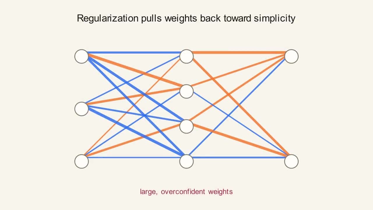
A small network appears with thick, saturated blue and orange edges representing large weights, captioned "large, overconfident weights." Every edge then thins down toward a faint line as the caption changes to "regularization shrinks them toward zero." This is the visual core of L1/L2 regularization: a penalty that continuously pulls every weight back toward simplicity.
dashed = true curve · filled dots = training points · outlined dots = held-out test points · solid = degree-3 fit (a reasonable fit)
Watch training error fall almost every step as degree rises - it can always fit the 16 visible points better. Test error does not follow it down: past the simplest fits it climbs, and climbs sharply once the curve starts chasing noise it's never seen.
L2 regularization multiplies every weight by 0.9 on every step. L1 subtracts 0.1 from every weight on every step. After five steps, which has shrunk a weight of 0.05 more?
- aL2 - it acts on every weight proportionally
- bL1 - fixed subtraction is harsher on small weights
- cAbout the same
- dNeither - 0.05 is too small for either to touch
Commit to a guess, then open this
L1, and not by a little: it deleted the weight entirely on the first step, while L2 still has 0.029525 of it after five. The fixed 0.1 is twice the whole weight, so the subtraction would take it past zero and the implementation clips it to exactly 0, where it stays. That is what “L1 produces sparsity” means, arrived at by arithmetic. Now ask the same question about a weight of 2.0: after five steps L1 has taken 25% of it and L2 has taken 41%. The two penalties do not differ in strength - they differ in who they are strong against.
A model that’s too simple for the pattern it’s trying to learn does poorly even on the data it trained on - it’s biased toward an overly rigid assumption about the shape of the answer, called underfitting. A model flexible enough to fit its training data almost perfectly can end up fitting that data’s specific noise, not just its underlying pattern - high variance, meaning it does great on data it’s seen and poorly on data it hasn’t, called overfitting. With a fixed amount of training data, you can’t drive both down freely at the same time - more flexibility trades bias for variance.
Both penalties below have a knob, λ, deciding how seriously the network takes them. At λ = 0 the penalty does nothing and you have ordinary training. As λ grows, the network is increasingly willing to fit the data worse in exchange for smaller weights, and at a large enough λ it gives up on the data entirely and drives every weight to zero. Typical values sit between 0.01 and 0.0001, and λ is a hyperparameter, meaning it is not learned from the data; you pick it, train, check the validation score, and pick again.
L2 regularization pulls every weight gently toward zero, proportional to its own size - weights shrink smoothly but essentially never hit exactly zero. L1 regularization pulls every weight by the same FIXED amount regardless of size - small weights can get pulled all the way to exactly zero and stay there, effectively switching off that connection entirely.
A proportional tax and a flat charge
L2 is income tax: everyone pays 10% of what they have, so a weight of 2.0 pays 0.2 and a weight of 0.05 pays 0.005. Nobody is ever taxed to nothing, because 10% of a tiny amount is a tinier amount. L1 is a flat annual fee: everyone pays 0.1 regardless. The large weight barely notices, and the small weight cannot pay and is wiped out. That is the whole mechanism, and the blocks in rung 2 are the two tax bills, side by side, for five years.
Where it breaks downTax revenue goes somewhere. Nothing collects the shrinkage; the weights just get smaller.
WordsToo rigid, too flexible, and the knob between themWhy you would ever deliberately make a model worse at its own training data.Rung 01
A model that’s too simple does poorly even on the data it trained on: underfitting. A model flexible enough to fit its training data almost perfectly ends up fitting that data’s specific noise: overfitting, which is high variance. With a fixed amount of training data, more flexibility trades bias for variance and you cannot drive both down at once.
A network with large weights can carve an overly wiggly decision boundary that memorizes training noise instead of the underlying pattern. Regularization adds a second goal to training beyond “minimize loss”: also keep the weights small. L2 pulls every weight toward zero in proportion to its own size. L1 pulls every weight by the same fixed amount regardless of size, which is why small weights can reach exactly zero and stay there.
One convention worth knowing because every framework implements it and few explanations mention it: regularization is normally applied to weights only, not biases. A weight controls how strongly two things are connected, and shrinking it toward zero means “care less about this connection”, which is a meaningful thing to want. A bias just shifts a neuron’s threshold; shrinking it toward zero means “prefer a threshold of exactly zero”, which is not something you have any reason to prefer. Biases are also few in number, so penalising them buys almost nothing.
NumbersThe decomposition, and five steps of each penaltyEvery claim on this page, as arithmetic, at the same lr and lambda the demo uses.Rung 02
Formally, the expected squared error decomposes into three parts, where E[…] means “the average value you’d get if you repeated this over and over”:
Illustrative example, not from real data: imagine training each model twice on two different samples of the same data, and both times predicting the same input, whose true value is 0.7.
The flexible model is right on average and wrong every single time. It is never retrained into the version whose prediction is 0.7; it produces 0.2 or 1.2 depending on which noisy sample it happened to see, and you only ever get one of them. That is what “zero bias, high variance” means in practice, and it is why the model with the wrong average beats it here.
Note that the two decompositions agree with the direct calculation exactly, in both cases. That is not luck, it is the identity the formula states; the noise term is zero here only because this example has no measurement noise in it.
Here are both penalties inside a full update, with the data gradient present, so the two forces are visible at once. One weight w = 0.80 (positive, blue), one input x = 1.0, target y = 0.50. The lr = 1.0 and λ = 0.1 are a deliberately exaggerated pair, the same one the demo below uses, both far larger than anything you would train with, chosen so every step is legible in four decimal places.
The data gradient was +0.30 in all three rows, and it wanted the weight smaller anyway, because the prediction was too high. The penalty added to it. (The unregularized row lands on exactly 0.5000, the target, which is an artefact of lr = 1.0 meeting x = 1.0 and not a general property; at a realistic learning rate it would land short.) Had the data gradient been negative, wanting the weight larger, the penalty would have fought it, and the weight would have settled wherever the two forces balance. That balance point, not zero, is where a regularized weight ends up.
The single most-repeated claim about L1 is that it drives weights to exactly zero and L2 does not. Here is that happening, with the data gradient set to zero so the penalties are isolated, at the same lr = 1.0 and λ = 0.1, on three weights of very different sizes.
Those last two rows are sparsity, arrived at by arithmetic rather than by assertion. L1 takes the same 0.1 from every weight, which is 5% of a weight of 2.0 and more than the whole of a weight of 0.05, so small weights are the ones that run out, and they run out in order of size: 0.05 is gone after one step, 0.5 after five, and 2.0 would need twenty. Once a weight hits exactly 0 the clipping holds it there, and that connection is switched off for good. L2 takes the same percentage from every weight, so a weight approaching zero has less and less taken from it and never arrives.
The clipping is not an implementation detail; it is what makes L1 work. The w = 0.05 row is the case worth pointing at: one step would take it to −0.05, then the sign of the penalty would flip, and it would oscillate across zero forever without ever landing on it. Real implementations use a proximal step, which is the clip written formally: take the ordinary gradient step, then move the weight toward zero by lr·λ and stop if you reach zero.
PictureTwo weights racing to zero, and a curve chasing noiseWhat proportional shrinkage and fixed shrinkage look like as motion.Rung 03
Set w₀ to 0.50 and press ‘Take 5 decay steps’ twice. The blue L2 dot has moved from 0.5000 to 0.2952 to 0.1743 and its steps are visibly shrinking as it approaches the dashed zero line, which it will never touch. The orange L1 dot went 0.5000 → 0.4 → 0.3 → 0.2 → 0.1 → 0 in five equal strides and then stopped dead on the line, and its readout changed to “(locked at exactly 0)”. Equal strides against shrinking strides is the entire difference between the two penalties, drawn.
Both paths use the same exaggerated lr=1.0, λ=0.1 as the worked example above (η=learning rate, λ=regularization strength). L1's steps are constant-size regardless of how close w already is to 0 - that's what lets it land exactly on 0 and stay there.
Back on the bias-variance demo in Figure 02: at degree 3 the solid curve tracks the dashed true curve and ignores individual dots. At degree 12 it passes through nearly every filled dot and misses the outlined ones by a mile - and the outlined dots are the only ones that matter, because they are the data the model never saw.
EquationThe two penalties and their gradientsTwo formulas, two gradients, and the factor the name comes from.Rung 04
L2 adds (λ/2)‖w‖² to the loss, contributing a gradient of λw, so an SGD update becomes w ← (1−ηλ)w − η∇loss. The (1−ηλ) factor is literally where the name “weight decay” comes from. L1 adds λ‖w‖₁ to the loss, contributing a constant-magnitude gradient of λ·sign(w).
Those double bars are the two penalties written compactly: ‖w‖₁ is the sum of all the weights’ sizes ignoring sign, and ‖w‖² is the sum of their squares.
General caseBoth at once, and why any of this smooths a boundaryThe third member of the family, and the sentence that connects the top of this page to the bottom.Rung 05
Elastic Net is both penalties at once, λ₁‖w‖₁ + (λ₂/2)‖w‖², and it exists because the two failure modes are different. L1 on its own, given several correlated inputs carrying the same information, tends to pick one of them arbitrarily and zero the rest, and which one it picks can change between training runs. Adding a little L2 makes it share the weight across the group instead. You get L1’s ability to switch connections off and L2’s stability about which ones.
And the link back to the top of this page, which is worth making explicit. Small weights produce a smoother decision boundary for a mechanical reason: a neuron’s output changes by w for every unit its input changes, so a large weight means a small change in the input produces a large change in the output, which is what a sharp, wiggly boundary is made of. Halve every weight in a layer and you halve how fast its output can swing. Regularization does not know anything about boundaries or overfitting; it only makes weights smaller, and smoother boundaries are what smaller weights look like when you plot them.
This connects directly to AdamW on the optimizers page: naively combining L2 regularization with an adaptive optimizer like Adam distorts the decay unevenly per parameter, which is exactly the problem AdamW’s decoupled weight decay fixes.
Why this and not that
Why penalise big weights rather than counting them?
Counting is not differentiable: a weight is either counted or not, so nudging it changes nothing until it crosses a threshold and then everything at once. There is no gradient to descend. L1 is the closest differentiable-almost-everywhere stand-in for counting, which is exactly why it is the one that produces genuine zeros.
Why is L2 the default when L1 gives you feature selection for free?
Because a sparse network is rarely what you want from a neural network, and L1’s arbitrary choice between correlated inputs makes runs less reproducible. L2 is smoother, easier to optimise, and pairs cleanly with the (1−ηλ) decay form that every optimizer implements. L1 earns its place where you genuinely want to switch inputs off.
If regularization makes the training error worse, how can it be helping?
Because the training error is not the thing you care about. Rung 2’s decomposition is the argument in numbers: the flexible model has zero bias and 0.25 total error, the rigid one has a large bias and 0.17. Accepting more bias to remove more variance is a net win whenever the variance was the larger term, which on small datasets it usually is.
Should λ be the same for every layer?
Usually yes, because you have no principled basis for varying it and every extra hyperparameter is another sweep. The exception that is not optional is biases, which are conventionally excluded entirely - and normalization layers’ γ and β, which are excluded for the same reason.
Is dropout a kind of L2?
They are not the same thing, but they are not unrelated either: for a simple linear model, dropout can be shown to be equivalent to an L2 penalty with a particular per-weight scaling. For a real network they behave differently enough that people use both, and the next page is the family dropout belongs to.
- L1 and L2
- The L is for Lebesgue, after Henri Lebesgue, whose name the ℓᵖ spaces carry. ‖w‖₁ is the ℓ¹ norm and ‖w‖₂ the ℓ². The names are pure functional analysis and say nothing about neural networks, which is why they look so arbitrary here.
- Norm
- From Latin norma, a carpenter’s square, hence a standard for measuring against. A norm is any consistent way of turning a list of numbers into one non-negative size.
- Weight decay
- Literally the (1−ηλ) factor: every step, the weight decays to a fixed fraction of itself, exactly like radioactive decay, and by the same arithmetic.
- Regularization
- From making a function “regular”, meaning well-behaved and smooth. The term comes from Tikhonov’s 1943 work on ill-posed problems, where adding a penalty was a way of making an unstable problem have a stable answer. Nothing to do with rules or regulation.
- Lasso
- Least Absolute Shrinkage and Selection Operator, Tibshirani 1996. The acronym was reverse-engineered onto the rope, and the “selection” is the sparsity in rung 2.
- Ridge regression
- L2 by its statistics name, from the ridge that appears in the response surface the method was originally developed to analyse.
- Elastic Net
- Both penalties at once, named for a net that stretches: it keeps the whole correlated group rather than letting one member escape with all the weight.
- What is happening
L2 multiplies by
(1 − ηλ) = 0.9every step, so after 25 steps the weight retains0.9²⁵ = 7.2%of itself, and after 250 steps it retains0.9²⁵⁰, which is tiny and is not zero. A weight of 0.0036 is still a live connection with a live gradient. The widget states the distinction in its own readout: “(asymptotes toward 0, never reaches it)” against “(locked at exactly 0)”.- Fix
If you want zeros, use L1, or prune explicitly by thresholding after training. L2 is for smoothness, not for sparsity.
- Watch for
- The blue L2 dot visibly still short of the dashed zero line after five presses, while the orange L1 dot has been sitting on it since the first.
- What is happening
On a large weight the ordering reverses. L2 has removed 41% and L1 only 25%, because L1’s fixed 0.1 is a small fraction of 2.0 while L2’s 10% is not. L1 is not a stronger penalty than L2; it is a penalty with a completely different profile across weight sizes, brutal at the bottom and mild at the top.
- Fix
Pick the penalty by which weights you want to affect, not by which sounds stronger. If you want the large weights reined in, that is L2’s job.
- Watch for
- The blue L2 dot ahead of the orange L1 dot - the opposite of the ordering in M1, from the identical widget, one slider drag apart.
- What is happening
This widget runs at the deliberately exaggerated
lr·λ = 0.1, and twenty steps of it have taken a substantial weight of 1.5 down to 0.18 under L2 and killed it outright under L1. Real training runs for tens of thousands of steps. A λ that is an order of magnitude too large does not make the model slightly simpler; it drives the network to the zero function.- Fix
Sweep λ over powers of ten - 0.01, 0.001, 0.0001 - and pick on validation score. Typical values live in that range, and the 0.1 here is a teaching value, flagged as such in rung 2 and in the widget’s own caption.
- Watch for
- Twenty steps of decay leaving 12% of a substantial weight, from a penalty that is supposed to be a gentle nudge.
- What is happening
The degree-12 fit is 172 times better on the data it was shown and about two and a half times worse on the data it was not: train 0.0021 against test 2.3594, where degree 1 scores 0.3614 and 0.9122. The training error fell for a completely real reason - the model genuinely does pass closer to those sixteen points - and that reason has nothing to do with the thing you wanted.
- Fix
Hold data out before you start, and make every decision on the held-out score. The next page is what you do with it once you have it.
- Watch for
- The solid curve threading through nearly every filled dot at degree 12, while the outlined test dots sit well off it.
- What is happening
One starting weight, one number of steps, one
lr·λ. Under L2 it is at 0.1743 and still a working connection; under L1 it has been at exactly zero since step five and that connection no longer exists. Swapping the letter in your config file changes the topology of the trained model, not just its smoothness.- Fix
Decide first whether you want a smaller model or a smoother one. If you want both, the answer is Elastic Net, and rung 5 says why the combination exists at all.
- Watch for
- The two readout lines from the same starting weight - one a number, one the words ‘locked at exactly 0’.
Both paths use the same exaggerated lr=1.0, λ=0.1 as the worked example above (η=learning rate, λ=regularization strength). L1's steps are constant-size regardless of how close w already is to 0 - that's what lets it land exactly on 0 and stay there.
dashed = true curve · filled dots = training points · outlined dots = held-out test points · solid = degree-3 fit (a reasonable fit)
Watch training error fall almost every step as degree rises - it can always fit the 16 visible points better. Test error does not follow it down: past the simplest fits it climbs, and climbs sharply once the curve starts chasing noise it's never seen.
- 01Find the largest starting weight that L1 can drive to exactly zero within ten steps.
Hint
L1 removes
lr·λ = 0.1per step.Answer
1.00, which reaches zero on step ten exactly. Anything above needs more steps - 2.0 needs twenty - and anything below arrives sooner. The rule is simply
w₀ / 0.1steps, because the step size does not depend on the weight at all. That linearity is L1. - 02Set w₀ to 2.0 and find the step count at which L2 first overtakes L1 - that is, the first step where L2’s weight is smaller than L1’s.
Hint
L2 keeps 90% per step; L1 removes 0.1 per step. Write both sequences out.
Answer
L2 is smaller from the very first step and stays smaller until L1 hits zero. Step 1: L2 1.8000 against L1 1.9000. Step 5: 1.1810 against 1.5000. Step 15: 0.4116 against 0.5000. Step 20: L1 reaches 0.0000 and L2 is at 0.2431, and from that step onward L1 is smaller forever. So there are two crossovers, not one, and which penalty is “stronger” depends entirely on when you look.
- 03Using the demo, demonstrate that L2’s shrinkage is the same percentage for every weight.
Hint
Run two different starting weights for the same number of steps and divide.
Answer
w₀ = 2.0 for five steps gives 1.180980, and
1.180980/2.0 = 0.590490. w₀ = 0.5 gives 0.295245, and0.295245/0.5 = 0.590490. w₀ = 0.05 gives 0.029525, and again 0.590490. Identical to six decimal places, and it is0.9⁵ = 0.5904900. The starting weight cancels completely, which is why L2 can never reach zero from any starting point. - 04On the bias-variance demo, find the degree at which the training error first drops below 0.10, and say what the test error is doing there.
Hint
Drag up one degree at a time and read both numbers.
Answer
Around degree 9, where training error reaches 0.0631 and test error is 1.6727 - having risen from 1.0028 at degree 3. Two things to take from that. The training error’s fall is smooth and encouraging and completely uninformative. And the test error has not merely stopped improving, it has got substantially worse, which is what makes overfitting an active harm rather than a wasted opportunity.
- 05Argue from the two demos why “keep the weights small” and “draw a smoother curve” are the same instruction.
Hint
What does a large coefficient let a polynomial do between two points?
Answer
A curve’s steepness at any point is set by its coefficients: double them and the curve changes twice as fast for the same movement along the x axis. A degree-12 fit can only thread every dot by swinging violently between them, and swinging violently requires large coefficients - which is why the degree-12 curve in the demo leaves the plot’s vertical range near the edges while the degree-3 curve does not. Shrink the coefficients and the curve physically cannot swing that hard, so it stops being able to visit individual noisy points. Rung 5 states the mechanism in one line: regularization knows nothing about boundaries or overfitting; it makes weights smaller, and smooth is what small weights look like when you plot them.
- Hugging FaceThe Trainer’s default is weight decay applied through AdamW, and the config line every fine-tuning script carries is
weight_decay=0.01- the same lambda as rung 1, at a realistic value rather than this page’s teaching value of 0.1. - GenomicsL1 is used to pick a handful of predictive genes out of twenty thousand candidates, because the zeros are the answer: the genes L1 does not switch off are the shortlist. That is sparsity being used as the output rather than as a side effect.
L2 is a tax on every weight, and L1 is a flat fee. The tax never quite takes everything; the fee bankrupts the small ones.
Which weights you want gone decides which of the two you reach for.
Both penalties on this page change the loss formula, which means both of them apply the same pressure to every weight on every step, forever, whether or not the model is currently overfitting. Neither can tell you when the overfitting started, because neither is looking at data the model has not seen. And neither can do anything about a network whose problem is not the size of its weights but the fact that a handful of neurons have quietly taken over and the rest are along for the ride. The next page’s techniques do not touch the loss formula at all. They change the training procedure instead - what the network sees, when you stop, and what each layer is allowed to hand to the next one.