Vanishing Gradients
What happens when backpropagation's chained derivatives shrink to nearly nothing in early layers, and why it matters.
Five layers, and the bottom one never moves
Five layers. Every weight a perfectly ordinary 0.6. One backward pass.
Nothing was misconfigured. The weights are not large, the learning rate is not wrong, and the network is only five layers deep. It will train, the loss will fall, and the bottom half will still be roughly the random numbers it started with.
Before this page - 4 pages, and this one is the previous page’s consequence4
Backpropagation
the gradient reaching an early layer is a product of every local slope between it and the output. This page is that sentence, taken seriously.Activation Functions
sigmoid’s slope peaks at 0.25, tanh’s at 1.0, and ReLU’s is exactly 1 wherever it is active. Those three numbers are the page.Xavier and He Initialization
one of the standard fixes is there, and it is the same per-layer factor being aimed at 1Gradients and Gradient Descent
the “norm” the clipping block uses is the same length measurement defined there
Drag the depth slider from 2 to 8 and watch the last bar fall through four gridlines. Then drag the weight scale up past 1.0 and watch the bars flip direction. Both of those are the same multiplication.
 0:15
0:15What this animation shows
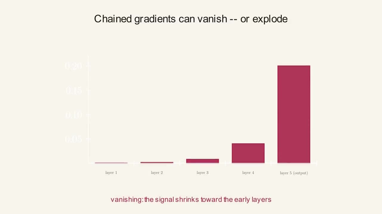
A bar chart of gradient magnitude per layer starts flat and near zero, then grows into a shape where each layer closer to the input is dramatically shorter than the last, captioned "vanishing: the signal shrinks toward the early layers." The chart then swaps to a mirror-image version where early-layer bars tower over the later ones, captioned "exploding: the same compounding, running the other way." This shows both failure modes the page covers as two sides of the same chained-multiplication problem.
This axis is log-scaled and centered on 1.0 - each gridline above center is a ×10 growth, each gridline below is a ×10 drop, because the real values shrink or grow so fast that on an ordinary axis every bar past the second one would look like it's touching zero or flying off the top.
At weight scale ≈1×, each layer's factor sits right at the tipping point between the two regimes - nudge the slider either direction to see which way it goes.
Five sigmoid layers. What fraction of the gradient reaches layer 1?
- aAbout a tenth
- bAbout a hundredth
- cAbout a thousandth
- dAbout a hundred-thousandth
Commit to a guess, then open this
About a hundred-thousandth - 0.0000610, which is 0.0061%. And the reason it is that small rather than the 0.00032 usually quoted is worth having straight away. The per-layer factor is not sigmoid’s slope on its own. Each layer multiplies by the slope and by the weight. Here the slope is about 0.24 and the weight is 0.6, so the factor is 0.145, not 0.24. A figure quoted as a power of the slope alone has told you half of a multiplication.
The backpropagation walkthrough showed that the gradient reaching an early layer is a product of every local slope between that layer and the output. Multiplying several numbers that are each less than 1 makes the result smaller every single time you add another one to the chain.
Sigmoid’s slope has a hard ceiling of 0.25, reached only at z = 0, and it falls away fast on either side: 0.1966 at z = 1, 0.1050 at z = 2, 0.0031 at z = 5.77. That gives two figures worth holding onto. In the best imaginable case, where every layer sits exactly at the peak and every weight is exactly 1, five layers give 0.25⁵ = 0.00098, under 0.1% of the original gradient; that is the optimistic bound and it is already bad. In the case usually quoted as typical, a pre-activation of about 1 with weights near 1, the slope is 0.1966, close enough to 0.2 that the figure gets written 0.2⁵ = 0.00032, and that is exactly what the demo shows at its default settings. The trace in rung 2 comes in lower still, at 0.0000610, sixteen times below the optimistic bound and five times below the typical one, for no reason other than its weights being 0.6 rather than 1. Sigmoid cannot avoid any of this; the ceiling is built into its shape.
Chinese whispers with a volume knob
Five people in a line. Each one passes the message on at 20% of the volume they heard it. By the front there is nothing to act on - not a garbled message, an inaudible one. Now imagine each person passes it on three times louder instead: by the front it is 243 times the original, which is not a message either. The people are layers, the volume multiplier is the slope times the weight, and the person at the front is the first layer, which is the one deciding what raw features the whole network is built on.
Where it breaks downIn the game the message also gets distorted. Here it is exactly the right message, scaled to nothing, which is worse - a distorted message can still be acted on, a zero cannot.
WordsOne multiplication per layer, done five timesWhy depth is a multiplication problem, and the two directions it fails in.Rung 01
The gradient reaching an early layer is a product of every local slope between that layer and the output. Multiplying several numbers that are each less than 1 makes the result smaller every single time you add another one to the chain.
Sigmoid’s slope has a hard ceiling of 0.25, reached only at z = 0, and it falls away fast on either side: 0.1966 at z = 1, 0.1050 at z = 2, 0.0031 at z = 5.77. The optimistic bound over five layers is 0.25⁵ = 0.00098; the usually-quoted typical case is 0.2⁵ = 0.00032, which is what the demo shows at its defaults.
ReLU’s slope is exactly 1 whenever it’s active, so a chain of active ReLU units multiplies 1×1×1×1×1=1, no depth-driven shrinkage at all. But that’s not the whole story: a ReLU neuron that’s always inactive has slope exactly 0, and once that happens it stops learning permanently, a “dead ReLU.” ReLU trades gradual vanishing for a different failure mode, not a free pass.
Vanishing has a mirror image: exploding. The chain rule doesn’t just multiply activation derivatives together - at each layer it also multiplies in that layer’s outgoing weight. If the weights are large, the per-layer factor can climb above 1, and the exact same compounding multiplication that made the gradient vanish now makes it explode.
NumbersA real backward pass through five real layersThe actual arithmetic, forward and backward, plus what each layer’s weight really receives.Rung 02
Before any powers of anything, here is a real gradient shrinking in a real network, computed the same way as the backpropagation walkthrough. The network is deliberately as simple as it can be while still being deep: five layers, one sigmoid neuron each, every weight set to 0.6 (positive, so blue), every bias 0, input 1.0.
Now backward. Start with a gradient of 1.0 arriving at the output, and pass it through each layer. The gradient travels from the last layer to the first, so this block and the lists below it run layer 5 first, the reverse of the forward table. Each pass multiplies by that layer’s slope, then by the weight:
Five layers, and 99.994% of the signal is gone. Nothing unusual was done to produce that; the weights are a perfectly ordinary 0.6 and the network is only five layers deep.
Look at what the per-layer factor is actually made of, because this is where most explanations quietly cut a corner. It is 0.145, not 0.24. Sigmoid’s slope contributes about 0.24, and the weight contributes 0.6, and it is their product that gets multiplied five times.
That also explains why the demo on this page reports a different number. It runs at a weight scale of 1.0 and a pre-activation of 1.0, so its per-layer factor is sigmoid’s slope on its own, sigmoid'(1.0) = 0.1966. This trace uses a weight of 0.6, so its factor carries that 0.6 as well and comes out at 0.145. Neither is wrong; they are two settings of the same knob, and the demo’s weight-scale slider is exactly the knob that moves between them.
“The training signal has all but disappeared” is worth converting into something you can picture. Here is what each layer’s weight actually receives from that single backward pass, at lr = 0.1:
That number, 1,401×, is the practical meaning of vanishing gradients. The network is not broken and it is not frozen; the last layer is learning at a normal speed while the first layer is effectively standing still. And the first layer is the one deciding what raw features everything else is built on. You get a network that trains, produces a falling loss, and has a bottom half that is still essentially the random numbers it was initialised with.
The fix has to change the per-layer factor, so it is worth seeing what each activation function contributes to it. Same five-layer network, same w = 0.6, same input, and the factor lists again run layer 5 first:
tanh beats sigmoid because its maximum slope is 1.0 rather than 0.25, four times higher, and that factor of four compounds. ReLU’s slope is exactly 1 wherever it is active, so its per-layer factor is the weight and nothing else, and the last row is the case everyone quotes: with weights near 1, the gradient passes through untouched. This is the entire argument for the ReLU family, now with the numbers behind it, and the dead-ReLU caveat is the price.
And the mirror image, in numbers. A per-layer factor of just 3, which one bigger weight is all it takes to produce, compounding over 5 layers gives 3⁵ = 243. Over 10 layers it is 3¹⁰ = 59,049. The update to a weight becomes a wild, oversized jump instead of a careful nudge, and training can diverge outright - loss shooting up instead of down, or turning into NaN.
PictureEight bars on a log axisEvery claim in rung 2, as a slider you can move.Rung 03
The axis in Figure 02 is log-scaled and centred on 1.0, so every gridline is a factor of ten and growth and shrinkage are mirror images rather than two unrelated pictures. At the defaults - sigmoid, depth 5, weight scale 1.0 - the per-layer factor reads 0.1966 and the final value 2.9e-4, which is the 0.2⁵ figure in rung 1 rather than the trace’s 0.0000610, because this widget runs at weight scale 1.0 and the trace runs at 0.6. Both are correct and rung 2 says why.
Now change one thing at a time. Depth 5 to 8: the last bar drops three more gridlines. Sigmoid to tanh: every bar rises, because tanh’s slope at the same point is 0.41997 rather than 0.19661, more than double. Tanh to ReLU: the bars go flat, all at exactly 1.0, because ReLU’s slope is exactly 1 and the factor is the weight scale and nothing else. Tick ‘Make some neurons dead’: the bars go to zero and stay there, and the readout says “blocked by a dead neuron” - not small, blocked.
The weight scale slider is what turns this from two separate demos into one: at 1×, it reproduces the vanishing behavior from the top of this page exactly. Push it below 1× and the bars shrink faster - smaller weights, faster vanishing. Push it above 1× and the bars flip to growing instead - the chart is centered on 1.0 specifically so growth and shrinkage read as mirror images of the same underlying multiplication, not two unrelated phenomena.
EquationThe per-layer factor, and clippingOne expression, and the one line of arithmetic that caps an explosion.Rung 04
There is one expression on this page and everything else is a consequence of it. The gradient reaching layer k from the output is the product, over every layer in between, of that layer’s activation slope times that layer’s outgoing weight. Two ingredients per layer, multiplied, then multiplied again across layers.
The standard fix for the exploding side is blunt and effective: gradient clipping. Before applying an update, check the size (the norm) of the gradient vector; if it’s above some threshold, rescale the whole vector down to that threshold before taking the step. Direction is preserved, only the size is capped. It doesn’t fix whatever’s causing the explosion, but it stops one enormous update from wrecking days of otherwise good training, which in practice is usually enough.
Clipping is one line of arithmetic, so here it is performed. The “norm” of a gradient is the same length measurement from the gradient descent page: square every component, add, take the square root.
Every component was multiplied by the same 0.322078, which is why the direction is preserved exactly. That is the difference between clipping by norm and clipping each component separately at some value: the latter changes the direction of the update, the former only its length. Norm clipping is the one used in practice, and clip_grad_norm_ is the function you will see in real training code.
General caseThe whole toolkitFive fixes, four of them already on this site, and why real networks use them together.Rung 05
Clipping stops explosions and does nothing for vanishing. Four other things do, and all of them appear elsewhere on this site, which is worth collecting in one place because a reader finishing this page is entitled to know that the problem has been solved rather than just described.
Two of those have their own pages here: scaled initialisation and normalization layers. Residual connections are covered in the convolutional networks module.
The reason to know all five rather than just the first is that they attack the same multiplication from different sides, and deep networks in practice use several at once. A modern residual network uses He initialisation, ReLU-family activations, normalization layers and skip connections together, and each one is aimed at the same product of per-layer factors that this page has been computing.
Why this and not that
If sigmoid is this bad, why was it ever used?
Because for a two- or three-layer network it is fine - 0.1966² = 0.039, which is a real loss and a survivable one - and because it outputs a probability, which is genuinely what you want at the output layer. Sigmoid is still correct for binary output. It is its use in every hidden layer of a deep network that the numbers here rule out, and that use is precisely what stopped in about 2011.
Why not just use a much larger learning rate for the early layers?
People have tried, and it is fragile: the factor by which the gradient shrank is not known in advance, it differs per layer, and it changes as training moves the weights. You would be tuning a per-layer learning rate against a moving target. The fixes in rung 5 change the factor itself rather than compensating for it, which is why they won.
Is exploding just vanishing with a bigger number?
Same mechanism, opposite side of 1, and completely different symptoms. Vanishing is silent: the loss falls, nothing errors, and the early layers quietly do not learn. Exploding is loud: one enormous update, then NaN, then the run is over. The loud one is far easier to diagnose, which is why clipping - a blunt fix for the loud problem - is standard, and there is no equivalent one-liner for the quiet one.
Does clipping fix vanishing too?
No, and rung 5 opens by saying so. Clipping caps a gradient that is too large; it does nothing whatsoever to a gradient that is too small. A threshold of 5.0 leaves a gradient of 0.000061 exactly as it was - the block in rung 4 shows a small gradient passing through completely untouched, which is the design.
If residual connections solve it, why is anything else needed?
Because a residual connection gives the gradient a path with a factor of exactly 1; it does not remove the other path, which still has all the same multipliers. Deep networks in practice stack several fixes: He initialisation, ReLU-family activations, normalization layers and skip connections, all aimed at the same product. Each one moves the factor closer to 1 by a different route.
- Vanishing gradient
- Named in Sepp Hochreiter’s 1991 diploma thesis, which analysed exactly this product and is the direct ancestor of the LSTM. The word is literal: the gradient does not become wrong, it becomes absent.
- Exploding gradient
- The mirror term, coined for the same product on the other side of 1. Both names describe what the number does, not what causes it, which is why they get used for symptoms with several different causes.
- Clipping
- From signal processing, where a signal that exceeds a range is clipped flat at the boundary. Gradient norm clipping is a gentler relative: it scales the whole vector down rather than flattening any component, which is why the direction check in rung 4 matters.
- Norm
- Latin norma, a carpenter’s square: a standard to measure against. Here it is the ordinary distance formula, the same one the gradients page used to combine two numbers into one.
- Dead ReLU
- A unit whose input is negative for every example in the dataset. Its slope is exactly 0, so its gradient is exactly 0, so its weights never change, so its input stays negative. “Dead” rather than “sleeping” because there is no mechanism that can wake it.
- Residual connection
- The block learns the residual, the difference between its input and the desired output, rather than the output itself. The shortcut carries the input forward unchanged, which is also what gives the gradient a path with factor 1.
- What is happening
Sigmoid’s slope has a hard ceiling of 0.25, reached only at z = 0, and at a typical pre-activation of 1.0 it is 0.19661. Eight layers of that is two millionths. This is not a tuning problem and there is no learning rate that fixes it: multiplying 2.233e-6 by a larger number gives a larger number that is still, relative to the last layer’s update, nothing.
- Fix
ReLU or one of its family in the hidden layers. Keep sigmoid for a binary output layer, where it is exactly right.
- Watch for
- Eight bars marching down through five gridlines on the log axis, and the readout reporting ‘vanishing’.
- What is happening
Active ReLU units have slope exactly 1, so at weight scale 1.0 nothing shrinks - that is the case everyone quotes. An inactive one has slope exactly 0, and zero is not a small factor, it is an absorbing one. The gradient does not shrink through a dead unit, it stops. And nothing revives it: no gradient means no weight change, means the input stays negative, means no gradient.
- Fix
Leaky ReLU, PReLU or ELU, all of which have a small non-zero slope on the negative side. Also check the learning rate, since a single oversized update is the most common way a ReLU unit is killed in the first place.
- Watch for
- The bars going to the danger colour and flat-lining at the zero rule, with the readout replacing a number with the word ‘blocked’.
- What is happening
The gradient arriving at layer 1 is now 6,561 times what left the output. The compounding that was destroying the signal is the identical compounding now destroying the weights; only which side of 1 the factor sits on changed. There is exactly one value that does neither.
- Fix
Compute the scale rather than tuning it -
2/n_infor ReLU - and if the gradient is still too small at the right scale, the answer is a normalization layer or a residual connection, not a bigger number. Clip as a safety net, never as the fix.- Watch for
- The bars flipping colour and growing upward off the top gridline, and the verdict switching to ‘exploding’.
- What is happening
tanh is the better activation - its slope at the same point is 0.41997 against sigmoid’s 0.19661, more than double - and this configuration vanishes a thousand times harder than sigmoid at weight scale 1.0 did in M1: factor 0.0840 and 2.478e-9 over eight layers. The per-layer factor has two ingredients and the weight is one of them. Swapping activations while leaving the initialisation badly scaled changes the smaller of the two factors.
- Fix
Fix the initialisation first. It is a one-line change with a known correct value, and it moves the factor further than an activation swap does.
- Watch for
- tanh - the better activation - producing a worse number than sigmoid did, from the same widget three clicks earlier.
- What is happening
At depth 2 the gradient reaching the first layer is 3.9% of what left the output. That is a real loss and it is survivable; the prototype trains. At depth 8 it is 0.0002%, a seventeen-thousand-fold difference, from the identical activation and the identical weights. The failure is exponential in depth, so it is invisible at the depth people prototype at and total at the depth they ship.
- Fix
Prototype at the depth you intend to deploy, or at least check the gradient magnitude at the first layer before scaling up.
p.grad.norm()per layer takes one line.- Watch for
- 3.9% and 0.0002% from the same activation, one slider drag apart.
This axis is log-scaled and centered on 1.0 - each gridline above center is a ×10 growth, each gridline below is a ×10 drop, because the real values shrink or grow so fast that on an ordinary axis every bar past the second one would look like it's touching zero or flying off the top.
At weight scale ≈1×, each layer's factor sits right at the tipping point between the two regimes - nudge the slider either direction to see which way it goes.
- 01Find the shallowest sigmoid network at weight scale 1.0 that loses more than 99% of its gradient.
Hint
The per-layer factor is 0.1966. When does
0.1966^kfall below 0.01?Answer
Depth 3, where
0.1966³ = 0.0076, so 99.24% is gone. Depth 2 leaves 3.87%. Three layers is not a deep network by any standard, and sigmoid has already destroyed 99% of the training signal. That is the fact the ReLU family was adopted for. - 02Find every configuration in this widget whose per-layer factor is exactly 1.0000, and say what they have in common.
Hint
Read the factor line while changing the activation and the weight scale.
Answer
Exactly one: ReLU at weight scale 1.0. Sigmoid would need a weight scale of 5.09 and tanh 2.38; the slider stops at 3.0, so tanh at 2.4 is the closest either gets and it reads 1.0079. What ReLU-at-1.0 has that the others do not is a slope of exactly 1, so the factor is the weight scale alone with nothing multiplied into it. That is the whole argument for the ReLU family in one readout, and it is why He initialisation aims at exactly this configuration.
- 03Make the gradient explode with tanh, then explain why you cannot do it with sigmoid.
Hint
Compare each activation’s slope at the widget’s pre-activation of 1.0 against the slider’s maximum.
Answer
tanh explodes from weight scale 2.5 upward - factor 1.0499, and at 3.0 it is 1.2599, giving 6.350 over eight layers. Sigmoid cannot be made to explode at all here:
sigmoid'(1.0) = 0.19661, so the weight scale would have to exceed1/0.19661 = 5.09and the slider stops at 3.0, where the factor is still only 0.5898. Sigmoid is not merely worse than tanh - it is stuck on the vanishing side of 1 across the entire range this widget offers, which is a fair summary of its position in deep networks. - 04Reproduce the page’s own trace as closely as this widget allows, and account for the difference.
Hint
The trace in rung 2 gives 0.0000610 at w = 0.6. This gives 2.28e-5. Which quantity differs?
Answer
The widget computes the slope at a fixed pre-activation of 1.0, giving
0.19661 × 0.6 = 0.1180, and0.1180⁵ = 2.28e-5. The trace computes each layer’s real pre-activation from the forward pass - 0.600000, 0.387394, 0.357393, 0.353046, 0.352414 - where sigmoid’s slope is nearer 0.24, giving per-layer factors around 0.1454 and a product of 6.10e-5. The trace’s factors are larger because its pre-activations are closer to zero, where sigmoid is steepest. Both are correct; the widget is a fixed-point approximation and the trace is the real forward pass, and knowing which is which is the point of this task. - 05Perform the clipping arithmetic in rung 4 on a different gradient and confirm the direction is preserved.
Hint
Norm, then scale, then check the ratios between components.
Answer
Take
g = [+6.0, −8.0, 0.0]with threshold 5.0. Norm is√(36+64) = 10.0, above the threshold, so scale by5.0/10.0 = 0.5and the clipped vector is[+3.0, −4.0, 0.0]with norm exactly 5.0. Ratios to the first component:[1.0, −1.3333, 0.0]before and[1.0, −1.3333, 0.0]after. Every component was multiplied by the same 0.5, which is why the direction survives. Clip each component separately at 5.0 instead and you would get[5.0, −5.0, 0.0], a ratio of[1.0, −1.0, 0.0]- a different direction, and a different update. That is whyclip_grad_norm_and notclip_grad_value_is the standard.
- LSTM, 1997Hochreiter and Schmidhuber designed the LSTM cell specifically to defeat this multiplication, after Hochreiter’s 1991 thesis analysed it. Its constant-error path is a route through time whose per-step factor is near 1 by construction - the same fix as a residual connection, six years earlier and in the other direction.
- LLM trainingAlmost every large language model’s training loop calls
clip_grad_norm_onmodel.parameters()with a threshold of 1.0. That single line is the block in rung 4, run once per step, for months.
Whisper a message through five people who each pass on a fifth of what they heard. The person at the front hears nothing, and they are the one deciding what the message was about.
Change the fraction to one and the message arrives intact. Every fix on this page is a way of changing the fraction.
This page has been about the gradient’s journey backward through a network’s hidden layers, and every fix in rung 5 is about the middle of the network. None of them says anything about the two ends. The first layer receives raw data whose scale you did not choose, and the last layer has to produce an answer in whatever shape the task demands - a number, a probability, one of a thousand categories - and the activation you put there is not a free choice. Pick the wrong one and a perfectly healthy backward pass arrives at an output layer that cannot express the answer at all, however well it was trained.