Weight Initialization
Why weights can't all start identical, and what breaks when naive random initialization is used at scale.
Two thirds of a layer, already stuck
A hundred-neuron layer. Every neuron different, every weight random. Watch what its output actually looks like before a single training step has happened.
Nearly two thirds of that layer is already stuck, and training has not started. Every one of those neurons will receive a gradient of about four hundred-thousandths of whatever arrives, forever. Nothing on the previous three pages can rescue this, because there is nothing wrong with the loss, the gradient, or the optimizer.
Before this page - 3 pages needed, 1 symbol borrowed from later4
The Single Neuron
a pre-activation is one neuron’s weighted sum before its activation function runsLayers and the Forward Pass
“n inputs per neuron” and the idea that one layer’s outputs are the next layer’s inputsActivation Functions
the flat, near-zero-slope tails of tanh and sigmoid are the entire hazard on this pageBackpropagation
delta appears once, in rung 5’s symmetry block, meaning “how much the loss changes if this number changes”. That gloss is borrowed from the backpropagation page verbatim; you do not need to derive it to read the block.comes later
Leave the toggle on ‘Same’ and press ‘Take 5 training steps’ three times. Read the two rows of numbers, not the picture. Then switch to ‘Random’ and do it again.
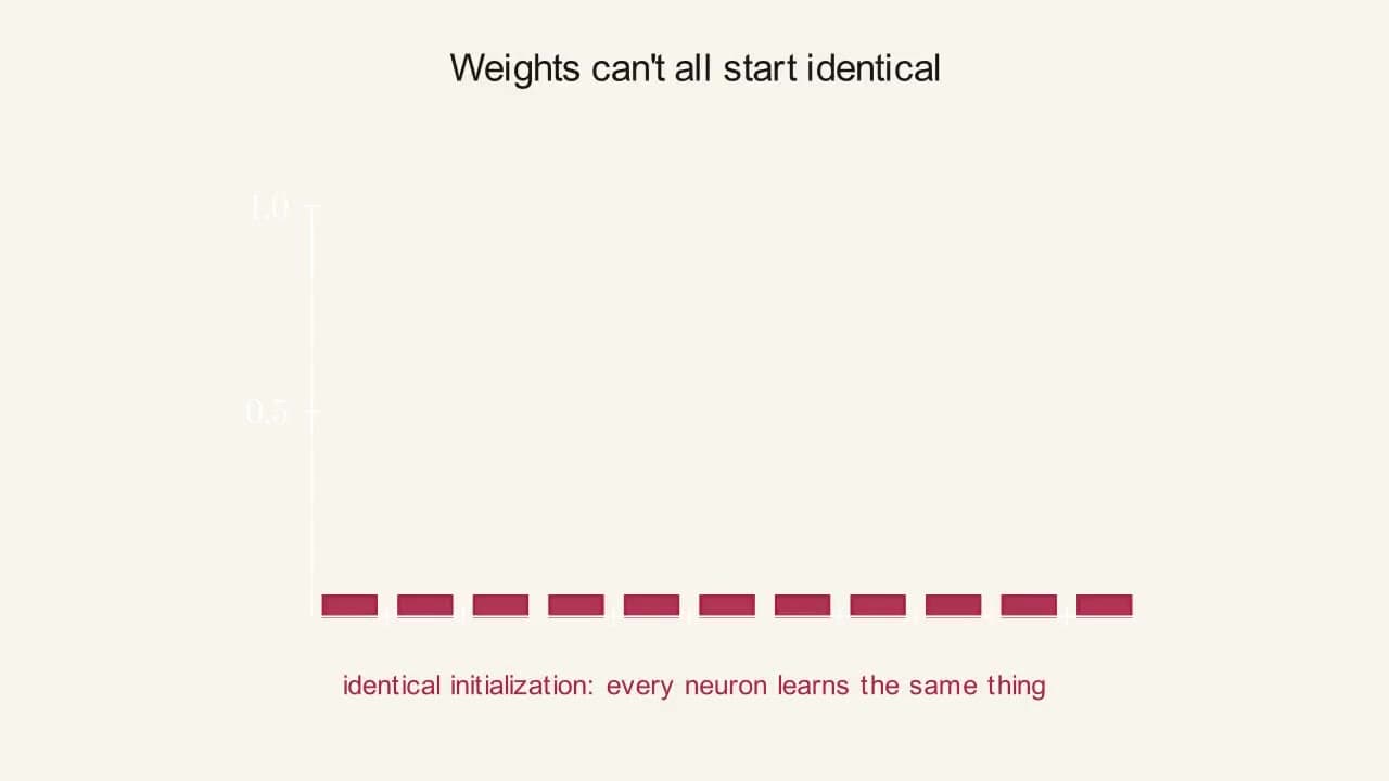 0:13
0:13What this animation shows
A histogram opens with every bar at the same tiny height, red, captioned "identical initialization: every neuron learns the same thing." The bars then reshuffle into a varied, randomly-spread set of heights in the site's accent color, with the caption changing to "random initialization: every neuron starts different." This is the page's opening problem made visible: weights can't all start identical, or every neuron in a layer computes the exact same thing forever.
With "Same," both neurons' weights change in exact lockstep, press after press, they're computing the same thing, so they get the same update. With "Random," watch the two rows above pull apart.
Both hidden neurons start with the identical weights. After fifteen training steps, how different are they?
- aSlightly different - training adds a bit of noise
- bVery different - fifteen steps is a lot
- cIdentical to several decimal places
- dIdentical to every decimal place, exactly
Commit to a guess, then open this
Identical to every decimal place, exactly, and they will be after fifteen million steps. This is not a rounding story or a slow-divergence story. The two neurons compute the same output, so they are told the same thing by the same backward pass, so they receive bit-for-bit identical updates. The widget’s readout says so in words: “Identical, still twins after 15 steps.” A layer of a hundred identical neurons is not a layer of a hundred neurons; it is one neuron, computed a hundred times, at a hundred times the cost.
If every neuron in a layer started out identical, they’d all compute the identical output for any input, get nudged by the identical amount during training, and stay identical forever, a whole layer of clones behaving like a single neuron in disguise.
Take two hidden neurons, h1 and h2, fed the same two inputs, started with the same weights and the same bias of 0 (this matches how the networks on this site actually initialize - bias starts at zero, weights don’t). Because they’re tied, h1 and h2 compute exactly the same output for any input you give them. Each neuron’s incoming weights then get nudged by how much that neuron’s own output contributed to the final answer being wrong, and since h1’s output and h2’s output are currently identical, that contribution is identical too, so their updates are identical. Twins stay twins, forever, no matter how much you train. That’s why bias is safe to start at zero, since it has no “which neuron am I” role to play, but weights must never be tied.
Why weights can’t all be the same size, either. Breaking the tie between neurons is only half the problem. Even with genuinely random weights, this site’s playground actually initializes every weight the same simple way: a fixed random draw between −1 and 1, regardless of how many inputs a neuron has (Math.random() * 2 - 1 under the hood). That fixed range turns out to matter a lot more than it looks.
An orchestra of one
Sit a hundred violinists down and give every one of them the identical part, the identical bowing and the identical tuning. You have not got a violin section, you have one violinist at a hundred times the volume. Worse, when the conductor corrects the section, every player makes the identical correction, so they stay one violinist forever. Randomising the starting weights is handing out a hundred slightly different parts.
Where it breaks downReal orchestras want players close to identical. Networks want them genuinely different, because the differences are where the capacity lives.
WordsDifferent from each other, and the right sizeTwo requirements, in plain language, and the one word this page is built on.Rung 01
If every neuron in a layer started out identical, they’d all compute the identical output for any input, get nudged by the identical amount during training, and stay identical forever. Twins stay twins. Bias is safe to start at zero, since it has no “which neuron am I” role to play, but weights must never be tied.
One word does most of the work from here on, so it is worth pinning down before it is used. Variance measures how spread out a set of numbers is. Take the numbers, find their average, measure how far each one sits from that average, square those distances, and average the squares. Numbers clustered tightly around their mean have a small variance; numbers scattered widely have a large one. The square root of the variance is the standard deviation, which is back in the original units and is usually the easier number to picture: it is roughly the typical distance from the average.
NumbersFive layers, twice, once too big and once too smallThe explosion and the collapse, layer by layer, with the tanh slope at the end of each.Rung 02
Both sets have the same average and behave completely differently inside a network. The average of a layer’s pre-activations tells you almost nothing useful; the spread tells you whether the layer is about to saturate.
For a neuron summing n inputs, each weight drawn independently with some variance σ², and inputs with variance 1: Var(output) ≈ n·σ². A fixed-range uniform draw between −1 and 1 has σ²=1/3, so as n grows, the output variance grows right along with it.
A typical pre-activation value is already around 5.77, well into sigmoid or tanh’s flat, saturated, near-zero-gradient territory, before training has taken a single step.
One layer reaching a typical size of 5.77 is a problem. The real problem is that the same multiplication happens again at the next layer, and the next. Each layer multiplies the incoming variance by n·σ², so across L layers the incoming variance is multiplied by (n·σ²)ᴸ.
By layer 2 every neuron in the network outputs either +1 or −1 and the slope of tanh at those values is zero to within floating-point precision. Zero slope means zero gradient, which means zero learning, forever. The network is dead before the first training step, and nothing about the training procedure can revive it.
Now the same arithmetic with weights drawn too small instead, variance 0.0001 rather than 1/3:
Same multiplication, different direction. The signal is gone by layer 5 either way. And there is a scale between them where the factor n·σ² is exactly 1 and the variance holds still at 1.0 forever, which for n=100 means σ² = 1/100. That number is not a coincidence and it is what the next page is about.
Flagged as simplified: this calculation treats each layer as a plain weighted sum and ignores what the activation function does to the variance on the way through. That is close to true for tanh while values are small, which is exactly the regime where the network is healthy, and it stops being true once values saturate, which is exactly the regime the calculation is warning you about. The activation’s effect gets handled properly on the next page, where it changes the answer for ReLU.
PictureThe histogram, at two widthsOne slider, and the moment a healthy layer becomes a dead one.Rung 03
The shaded bands are where tanh and sigmoid have gone flat. Drag n to 2 and the whole distribution sits between the bands: std 0.780, 0.0% in the flat zone, and this initialisation looks completely fine. Drag n to 20: std 2.545, 24.9% flat. To 100: std 5.773 - the same 5.77 the block above derived by hand, arrived at here by sampling a thousand neurons - and 62.2% flat. To 200: std 8.502 and 72.4% flat.
Nothing about the weights changed across that drag. Every weight is still a fresh draw from uniform(−1, 1). The only thing that changed is how many of them are being added together, and that alone decided whether the layer works.
Each bar is the share of 1,000sampled neurons whose pre-activation value landed in that range. The shaded bands mark roughly where sigmoid/tanh go flat (|x| > 3) - gradient close to zero there, before training even starts.
This is this site's actual current init: uniform(−1, 1), regardless of n. Drag n up and watch the spread grow with it.
Both directions are the same shrink-or-explode pattern you’ll see again, in a different form, on the vanishing-gradients page - here it’s happening on the forward pass, before training even starts, rather than on the backward pass.
EquationVar(output) ≈ n·σ², and where 1/3 comes fromOne formula, two symbols, and the fact that makes uniform(−1,1) equal 1/3.Rung 04
For a neuron summing n inputs, each weight drawn independently with variance σ², and inputs with variance 1: Var(output) ≈ n·σ².
Two symbols come with variance and standard deviation and are used from here to the end of the module. σ (sigma) is the standard deviation and σ² is the variance, which is why you will see the same quantity written both ways depending on which one the formula wanted. When a block says sigma^2 = 1/3, it means the variance of that set of weights is 1/3, so their typical distance from zero is √(1/3) = 0.577.
One more fact, because the number 1/3 appears three times without explanation above. Drawing a weight evenly from the range (−a, a) gives it a variance of a²/3, so uniform(−1, 1) has variance 1/3. That formula gets derived on the next page, where it also turns out to be where the mysterious 6 in Xavier’s uniform bound comes from.
General caseWhy twins stay twins, proved, and the named schemesThe twins argument computed rather than asserted, then every initialiser name you will meet in code.Rung 05
Written out with numbers, in the same 2-2-1 tanh network as the backpropagation page, with every weight in the network set to the same value 0.25 (positive, so every connection would be drawn blue) and every bias 0. Inputs x₁=0.50, x₂=−0.20, target y=1.
One symbol in the block belongs to that later page, so here is what it means, in that page’s own words. δ (delta) for a number is how much the loss changes if that number changes. δ_o is that quantity for the output neuron, δ_h1 for the first hidden neuron. The three lines under BACKWARD are the procedure that carries δ from the output back to the hidden layer, and deriving them is backpropagation’s whole job. You do not need to be able to derive them to read what this block shows, which is that the two hidden neurons’ numbers come out identical at every single stage.
Notice which numbers had to be equal for this to happen: the two hidden neurons’ outputs, because their incoming weights were equal, and then the two outgoing weights v1 and v2, which fed identical δ_o back to both. Break either one and the twins separate immediately. Random initialisation breaks both at once, which is why it is the standard fix rather than something more clever.
Every deep learning framework ships a menu of initialisers, and the names are more intimidating than the ideas. All of them are answers to the same two questions asked on this page: are the weights different from each other, and are they the right size? (n_in below is how many numbers arrive at each neuron in the layer; it gets a proper name, fan-in, on the next page.)
The last three are the ones you actually use, and they are the subject of the next page. The first two are worth knowing mostly so you recognise what has gone wrong when a network refuses to learn at all.
Why this and not that
Why is zero fine for biases and fatal for weights?
A bias has no “which neuron am I” role to play: two neurons with identical biases but different weights still compute different things. A weight is the only thing that distinguishes one neuron’s view of the input from another’s. Set the weights identical and the biases cannot rescue it; set the biases identical and the weights do the rescuing for free.
Why not initialise every weight to zero? It is the least biased choice.
It is the worst possible choice, and it is worse than “all the same non-zero value”. Every neuron is identical, so the twins problem applies, and every gradient flowing back through the layer is multiplied by an outgoing weight of zero, so it is zero. The layer receives no update at all, ever. Rung 5’s named-schemes block says this in one line, and the mistake mapper below has it as a preset you can run.
Does uniform versus normal matter?
Far less than people expect. What matters is the variance; the shape barely does. A uniform draw and a normal draw with the same variance produce layers that behave near-identically, which is why frameworks ship both versions of Xavier and He and nobody argues about which.
If the problem is the scale, why not just normalise the inputs and be done?
Input normalisation fixes layer 1. The five-layer block in rung 2 starts with an input variance of exactly 1.0 - already normalised - and still reaches 41 million by layer 5, because each layer multiplies the variance again. Normalising the input controls the number going in; initialisation controls the multiplier.
The page says this site’s own playground does it wrong. Why has it not been fixed?
Because the playground’s networks are tiny, and at n = 2 or n = 4 the fixed ±1 range is genuinely fine - the histogram shows 0.0% of a 2-input layer in the flat zone. The bug only exists at width. Naming what the site’s own code does, and where it stops being defensible, is the honest version of this page.
- Variance
- From Latin variare, to change. Fisher gave it its modern statistical meaning in 1918, and defined it as the square of the standard deviation rather than the other way round, which is why the squared quantity has the simpler name.
- σ, sigma
- The Greek s, for “standard deviation”. σ² is the variance for no better reason than that it is sigma squared.
- Fan-in, fan-out
- Borrowed straight from digital logic, where a gate’s fan-out is how many other gates its output can physically drive. A neuron’s fan-in is how many signals arrive; its fan-out is how many places its answer is sent.
- Symmetry breaking
- From physics, where a symmetric system settles into one of several asymmetric states. A layer of identical neurons is symmetric under swapping any two of them, and training cannot break that symmetry on its own; the random draw has to.
- Saturated
- From chemistry, by way of electronics: a saturated component cannot respond to more input because it is already at its limit. tanh(33.33) is 1.00000000 and tanh(3333) is also 1.00000000.
- What is happening
h1 and h2 compute the same output, so the backward pass sends them the same error signal, so they receive identical updates. The widget’s readout reports it directly: “Identical, still twins after 15 steps.” Adding neurons to this layer adds cost and no capacity.
- Fix
Draw every weight independently. Any distribution will do for breaking the tie; the next page is about which one gets the scale right as well.
- Watch for
- Both rows of the readout printing the identical three numbers, fifteen steps in. Then press the toggle to ‘Random’ and press it five times: ‘Diverged after 5 steps.’
- What is happening
This is worse than the previous one and for an extra reason. Every hidden weight stays at exactly 0.000, fifteen steps in, and so do both output weights. The output weights are zero, so
δ_h1 = δ_o · v1 · slopeis zero, so every first-layer gradient is zero. And the first-layer weights are zero, so both hidden outputs are zero, so∂L/∂v1 = δ_o · h1_outis zero too. The only parameter in the entire network with a non-zero gradient is the output bias. The network can learn to predict one constant and nothing else, forever.- Fix
Zeros are correct for biases and fatal for weights. Every framework’s default weight initialiser is non-zero for exactly this reason; if you are writing
torch.zeros_for a weight tensor, that is the bug.- Watch for
- Both readout rows reading (0.000, 0.000) → out weight 0.000 after fifteen steps. Not small. Zero.
- What is happening
Every weight is an honest independent draw from uniform(−1, 1). The problem is that two hundred of them are being added together, and adding two hundred independent numbers multiplies the variance by two hundred. Nothing about the weights is wrong; the sum is. This is the site’s own current initialisation, and at this width it puts nearly three quarters of the layer into the region where tanh’s slope is under 0.01.
- Fix
Scale the draw by the layer’s fan-in. That is the whole content of the next page.
- Watch for
- The histogram spilling into both shaded bands with only a thin spike left in the middle, and the flat-zone percentage rendering in the danger colour.
- What is happening
At n = 2 this initialisation is genuinely fine, and the histogram says so with a clean 0.0%. Every increase in width makes it worse, and the growth is
√n: doubling the width multiplies the spread by 1.414. Between n = 2 and n = 100 the spread grows 7.4×, and the failure appears somewhere in the middle, at a width nobody tested.- Fix
Test the initialisation at the width you will actually deploy, or better, size the draw so width cannot matter.
- Watch for
- 0.0% and 62.2% from the identical scheme, one slider drag apart.
- What is happening
This preset shows random initialisation doing its job perfectly: the twins separate immediately and stay separate. Now fire mistake 3 or 4 and look at the histogram: the identical initialisation, at a hundred inputs, has already saturated most of the layer. Breaking symmetry and getting the scale right are two different problems with two different failure modes, and solving the first tells you nothing about the second.
- Fix
Both, always. Independent draws and a variance sized to the fan-in.
- Watch for
- “Diverged after 15 steps” - the good news - sitting next to a 62.2% flat-zone reading from the same distribution.
With "Same," both neurons' weights change in exact lockstep, press after press, they're computing the same thing, so they get the same update. With "Random," watch the two rows above pull apart.
Each bar is the share of 1,000sampled neurons whose pre-activation value landed in that range. The shaded bands mark roughly where sigmoid/tanh go flat (|x| > 3) - gradient close to zero there, before training even starts.
This is this site's actual current init: uniform(−1, 1), regardless of n. Drag n up and watch the spread grow with it.
- 01Make the two hidden neurons diverge in as few steps as possible.
Hint
The button takes five steps at a time. How many presses does ‘Random’ need?
Answer
One. The readout switches to “Diverged” after the first block of five, and in fact they were different from step one - the widget only checks after you press. With ‘Same’ selected, no number of presses ever changes the verdict. Symmetry breaking is not gradual; it either happened at initialisation or it never happens.
- 02Find the layer width at which this site’s own initialisation first puts more than half the layer into the flat zone, to the nearest ten.
Hint
It is between 50 and 100. Read the flat-zone percentage as you drag.
Answer
Between n = 50 (46.9%) and n = 100 (62.2%), so it crosses 50% somewhere around n = 60. Predicting it: the spread is
√(n/3), so half the layer is beyond ±3 when√(n/3) ≈ 3/0.674, giving n ≈ 60. Sixty inputs is a small layer. The first layer of a network reading 28×28 images has 784. - 03Using only the histogram, estimate the std of the pre-activation at n = 100 and check it against the hand calculation on this page.
Hint
The widget prints the std. The page derives it in rung 2.
Answer
The widget reports 5.773 and the hand calculation gives √(100 × 1/3) = √33.3333 = 5.773503. They agree to four significant figures, which is what a thousand samples buys you. This is worth doing once: the formula in rung 4 is not a rule of thumb, and the histogram is not a cartoon, and they are computing the same number by two completely different routes.
- 04Set the network to all zeros and find the one parameter that still moves.
Hint
The readout shows six weights. It does not show all nine parameters. Which one is missing from it, and why would that one be different?
Answer
The output bias
bo. Its gradient isδ_o, which does not multiply by any weight or any hidden activation, so it is the only parameter in the network whose gradient survives when everything else is zero. The network converges to predicting a single constant - the best constant it can, which is a real if useless model - and every weight in it stays at exactly zero forever. - 05Argue, from the two blocks in rung 2, what per-layer variance factor would keep a 100-wide layer stable, and check it against the histogram.
Hint
The factor is
n·σ². What does it have to equal for nothing to change?Answer
Exactly 1, so
σ² = 1/n = 1/100 = 0.01, and std = 0.1. Checking it in the widget: the Xavier scheme on a square layer usesVar(W) = 1/nprecisely, and at n = 100 it reports std(pre-activation) = 1.018 with 0.2% in the flat zone - a layer whose output spread matches its input spread, which is the entire design goal. Compare naive’s 5.773 and 62.2% from the identicaln. That1/nis the next page.
- PyTorch nn.LinearIts default is Kaiming-uniform with
a = sqrt(5), not a fixed range - which is why a freshly constructed PyTorch layer already has weights sized to its own fan-in, and why you usually never have to think about any of this until you write an init by hand. - AlexNet, 2012Initialised its weights from a normal distribution with std 0.01 and set several biases to 1 specifically to keep its ReLUs firing early in training. The paper spells out the initialisation as a design decision, which is roughly when the field stopped treating it as an afterthought.
A layer of identical neurons is one neuron with an expensive accountant, and a layer of badly scaled neurons is a hundred neurons that have already stopped listening.
Different from each other, and the right size. Everything on this page is one of those two.
This page can tell you that n·σ² = 1 is the scale that holds still, and it can show you what happens either side of it. It cannot tell you what to do when a layer’s fan-in and its fan-out are different numbers, which is nearly every layer in a real network - sizing for one direction leaves the other drifting. And every calculation here treats a layer as a plain weighted sum, ignoring what the activation function does to the variance on the way through. That is close enough to true for tanh near zero, and badly wrong for ReLU, which throws away half its input. Both of those gaps have names, and both are the next page.