Gradients and Gradient Descent
What a gradient is and how repeatedly stepping downhill trains every weight in a network.
One number, two completely different runs
Same network, same data, same code. One number changed, and it did this.
The number that changed is not a weight and not a data point. It is not part of the network at all. This page is about what it is and why it has that much power.
Before this page - 2 pages, both immediately before this one2
Optimizers and vanishing gradients are forward links out of this page rather than dependencies into it, so they are linked in the prose below instead of listed here.
Loss Functions
this page starts from the one number that page produces and turns it into a weight change; the half-squared-error convention comes from there tooActivation Functions
the nudge-and-measure check on this page is the same one used to verify that page’s derivative table, so it should already look familiar
Take a step. Then take four more. Then drag the learning rate somewhere else and press Reset and do it again. Find, by experiment, the largest value that still gets to the bottom.
 0:14
0:14What this animation shows
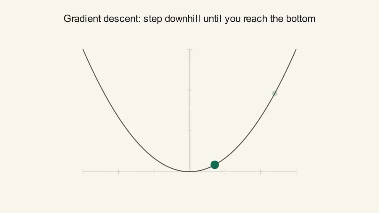
A ball sits partway up a parabola (loss(x) = x^2) and takes a series of discrete steps, each one rolling it further downhill, leaving a fading trail of ghost positions behind it. The ball's steps get smaller as it nears the bottom, and it settles at the minimum and turns green. This is gradient descent in miniature: repeatedly stepping in the downhill direction until you reach the lowest point.
This curve is the loss - height is how wrong the network is for a given weight value. Each step nudges the weight downhill. Faded circles are the last few positions, so you can see whether the ball is settling down or flying farther out.
The ball is at x = 2.4 and the slope under it is 4.8. To go downhill, does the next step add 4.8 to x or subtract it?
- aAdd - the slope is positive, so go that way
- bSubtract - the slope points uphill
- cNeither, it depends which side of the bowl you are on
Commit to a guess, then open this
Subtract. The slope always points in the direction the loss increases, in every dimension at once, so going downhill always means moving against it. At x = 2.4 the slope is +4.8 and the step is negative. At x = −2.4 the slope is −4.8 and the step is positive. You never have to check which side you are on; the sign of the gradient has already checked for you. That is why the update rule has a minus sign in it and why it needs no if statement, and it is the single most-asked question on this page.
Picture the loss as a landscape and a weight as a ball resting somewhere on that landscape - its height is how wrong the network currently is. The slope of the ground directly under the ball is called the gradient. Repeatedly nudging the ball a little in the downhill direction is gradient descent - it’s how every weight in a network gets better over time.
So far that has nudged one number. A network has thousands, sometimes billions, and each one has its own answer to “if I nudge you, how much does the loss change?” A gradient is nothing more than the whole collection of those answers, one per parameter, written down as a list.
Each entry is called a partial derivative, and “partial” just means you nudge one parameter while holding every other one perfectly still. Nudge w₁ alone, measure the loss change, write it down. Put w₁ back. Nudge w₂ alone, measure, write it down. The resulting list is the gradient.
Two pieces of shorthand, because everything from here on uses them. The entry for a parameter w is written dL/dw, said “d L by d w”, and it means precisely the nudge-and-measure number: how much the loss L changes per unit change in w. And lr is the learning rate, the fraction of that measured slope you actually move.
The list has a useful property that makes it worth calling a single object: read as a direction in the space of all the parameters at once, the gradient points in the direction of steepest increase of the loss. That is why the update rule has a minus sign in it. You want the loss to go down, the gradient points up, so you step against it. Every “why is there a minus sign there” question about training has that as its answer. It is also checkable, and rung 4 checks it.
Descending in fog
You cannot see the valley. You can feel the ground under one boot. Slide the boot around: whichever way it drops fastest is the downhill direction, and you step that way and repeat. The gradient is that slide, done once per parameter instead of once per boot. The learning rate is your stride length, and the argument about stride length is the argument this page is really about.
Where it breaks downA real hillwalker can see fifty metres ahead in patchy fog. Gradient descent sees precisely zero distance ahead; it only ever knows the tilt at the exact point it is standing.
WordsA list of tilts, one per parameterWhat a gradient is, in one sentence, plus why the update subtracts it.Rung 01
The loss is a landscape. A weight is a ball on it. The height of the ground is how wrong the network currently is, and the slope of the ground directly under the ball is the gradient. Step downhill, repeatedly, and the network gets better.
With more than one parameter there is no single slope, so there is a list of them, one per parameter. Each entry is a partial derivative: nudge that one parameter, hold every other one perfectly still, and write down how much the loss moved. Do that once per parameter and the list you end up with is the gradient.
Read as a direction rather than as a list, the gradient points in the direction of steepest increase of the loss. You want the loss to go down. The gradient points up. So you step against it, and that is the whole of the minus sign.
NumbersThree descents, worked by handOne parameter, then two, with every intermediate value printed.Rung 02
Take the simplest possible loss landscape, loss(x) = x². Its slope at any point turns out to be 2x, but rather than trusting a formula out of nowhere, check it the honest, no-calculus way: nudge x by a tiny amount and see how much the output moves.
That’s the honest, no-calculus definition of a derivative: how much the output changes for a tiny change in input, divided by that tiny change. Notice the answer came out to 6.001, not exactly 6 - the smaller the nudge, the closer this gets to the true slope; shrinking the nudge all the way toward zero is what calculus calls the derivative. This is the same trick already used to verify the derivative table on the activation-functions page, and it’ll come back once more on the output-activations page, so it’s worth having solid here.
One gradient descent step is just x_new = x − lr·gradient(x). Worked example: starting at x=2.4 with lr=0.35, the gradient is 2×2.4=4.8, so the next value is 2.4 − 0.35×4.8 = 0.72, much closer to the bottom (x=0) already.
Now the gradient of an actual loss with respect to two actual parameters, computed by hand. This is the same kind of network the loss functions page left off with, now taken the rest of the way: ŷ = w·x + b with w = 0.50 (positive, so blue on a diagram) and b = 0.00, on two training points. The loss is the average half-squared error, this site’s convention, which is why every gradient below comes out without a stray factor of 2 in it.
Three things to take from that. Both entries of the gradient were negative, so both parameters went up, and they went up by different amounts, because w had the steeper slope. Nobody decided that; it fell out of the arithmetic.
The “length” line is worth reading twice, because it is the first place on this site where two numbers get combined into one. It is the ordinary distance formula: square each entry, add, take the square root. That single number is how big the whole gradient is, ignoring which direction it points, and it is shrinking, which is what “approaching a minimum” looks like numerically: the ground under the ball is getting flatter. At an exact minimum, every entry of the gradient is 0, the length is 0, and the updates stop by themselves. This same quantity comes back on the vanishing gradients page under its other name, the norm, where clipping is defined in terms of it.
And look at how dL/dw got built: (−0.500000×1.0 + −2.000000×2.0) / 2. The second example contributed −4.0 of the −4.5 total, 89% of the whole signal, because its error was four times as large and its input was twice as large. Each example’s vote is weighted by its own error and its own input. Nothing about that is specific to this loss; it is what “the gradient of an average” means, and it is why one badly-fit example with a large input can dominate a whole batch.
PictureSix learning rates on one curveThe learning-rate claims, checked, and the same six runs on screen.Rung 03
Below about lr=0.5, the ball glides smoothly to the bottom. At exactly lr=0.5 it reaches the bottom in a single step. Between 0.5 and 1 it overshoots past the bottom and bounces to the other side, but each bounce is smaller than the last. At exactly lr=1, it bounces forever at the same distance, never settling and never escaping. Above lr=1, it overshoots farther every single step. Those claims are checkable, so here they are checked. Starting from x=2.4 on loss(x) = x², one step is x ← x − lr·2x = x·(1 − 2·lr). The whole behaviour is decided by that one multiplier.
The rule behind all six rows: the step converges when |1 − 2·lr| < 1, which for this landscape means lr < 1. The bars in |…| mean “ignore the sign”, so a multiplier of −0.80 counts as 0.80 and shrinks the number it multiplies, while −1.20 counts as 1.20 and grows it. The 2 in that expression is how sharply x² bends, its curvature: the slope of x² is 2x, which gains 2 for every 1 you move sideways, and a bowl whose slope changes faster means a smaller maximum safe learning rate. That is not a quirk of this toy function, it is the constraint that decides learning rates in real training, and it returns with real numbers on the optimizers page.
Every row of that table is a setting of the slider in Figure 02, and the fading trail is the row drawn. At lr = 0.10 the trail is a line of dots marching one way. At lr = 0.90 the dots alternate left and right of the bottom, each one closer in. At lr = 1.00 there are only ever two dots, because the ball visits exactly two places forever. Above 1.00 the trail runs off the edge of the frame and the ball sticks against it - at that point stop reading the picture and read the weight number underneath, which keeps going.
EquationThe update rule, and why it points that wayFive directions, the same step size, and the one that wins.Rung 04
One gradient descent step is x_new = x − lr·gradient(x), where lr controls how big a step to take.
The claim that the gradient points in the direction of steepest increase is the one the minus sign rests on, so here it is checked rather than asserted. Stand at the same starting point, w = 0.500000, b = 0.000000, where the loss is 1.062500. Move exactly the same distance, 0.1, in five different directions and see what the loss does. Each direction is written as “how much of the step goes into w, how much into b”, scaled so the total distance moved is 0.1 every time.
Every direction with a downhill component lowers the loss, and the one built from the gradient lowers it the most: 0.240292 against 0.231237 for the nearest competitor, and more than twice what moving b alone achieves. Turn the direction around and it becomes the single fastest way to make the loss worse, which is the same fact stated from the other side. That is what “steepest” means, and it is why the update subtracts the gradient instead of adding it.
General caseA million parameters, and where this stops workingSame arithmetic, longer list, and the two ways the friendly picture lies.Rung 05
Nothing about the five-direction check depends on the loss being squared error or on there being two parameters; with a million parameters the arithmetic is the same and only the list is longer.
Two honest limitations, because the picture above is deliberately friendly.
x² has exactly one minimum and gradient descent cannot fail to find it. A real loss landscape has many. It can have local minima, dips that are not the deepest dip available, and far more commonly it has saddle points, places that slope down in some directions and up in others, where the gradient is near zero in every direction and progress stalls without the loss being anywhere near as low as it could get. In very high-dimensional networks saddle points are the more serious of the two, simply because a point needs to curve upward in every one of a million directions at once to be a true local minimum, and that is rare. Most of what optimizers do beyond plain gradient descent is about getting through flat and awkward regions faster.
And nothing here says when to stop. Gradient descent has no built-in finish line; the gradient shrinks toward zero but never quite arrives. In practice you stop after a fixed number of steps, or when the loss stops improving, or when a separate held-out score stops improving, which is early stopping.
Why this and not that
Why not just solve for the minimum? We know the formula.
For x² you can, and the answer is x = 0. For a network you cannot: there is no closed-form solution for where a million-parameter non-linear loss is smallest, and even for the cases where linear algebra could do it, inverting a million-by-million matrix is far more expensive than taking a few thousand cheap steps.
Why a fixed step size rather than jumping straight to the bottom?
Because the gradient only tells you the tilt where you are standing, not how far the bottom is. The size of the gradient is a hint about that, which is why plain gradient descent takes big steps far out and small steps near the bottom for free. Methods that do try to estimate the distance exist - they use the curvature, the rate at which the tilt changes - and they are usually too expensive for networks this size.
Why is 6.001 acceptable? That is not 6.
It is the honest answer to the question we actually asked, which was “how much does the output move for a nudge of 0.001”. Shrink the nudge to 0.0001 and you get 6.0001. The derivative is what that sequence approaches, not any one member of it. Real autodiff does not do this arithmetic at all; it applies exact formulas that someone derived once by taking that limit properly.
If the gradient is zero, is training finished?
It means training has stopped, which is not the same thing. A zero gradient happens at the bottom of a bowl, at the top of a hill, and at a saddle point, and in a high-dimensional network the saddle point is by far the most likely of the three.
Everyone says gradient descent finds the global minimum. Does it?
No, and it mostly does not matter. Large networks have vast numbers of local minima and, empirically, most of the reachable ones are about equally good. The failures that hurt in practice are flat regions and badly scaled directions, which is what the next page’s optimizers exist for.
- Gradient
- From Latin gradus, a step, via the 19th-century engineering sense of a road’s gradient: how much you climb per unit you travel. Same meaning, more dimensions.
- Descent
- Because you go down. It is named after the direction of travel, not the mechanism, which is why the mirror-image procedure for maximising something is called gradient ascent and is otherwise identical.
- ∂
- A “curly d”, written that way purely to distinguish a partial derivative (nudge one thing, hold the rest still) from an ordinary one (there is only one thing). It is read “partial”, or often just “d”.
- η
- The Greek letter eta, the near-universal symbol for a learning rate in papers. There is no story: it was a free letter. Code almost always calls it lr instead.
- Learning rate
- It is the fraction of the measured slope you actually move. Not a speed, not a percentage of anything else, and nothing in it is per second.
- Saddle point
- From the shape of a horse’s saddle: curving down along the horse and up across it, so the flat point in the middle is a minimum in one direction and a maximum in the other.
- What is happening
One step is
x ← x·(1 − 2·lr). At lr = 1.10 that multiplier is −1.20, so the ball crosses the bottom and lands 20% further out than it started, every single time, forever. Nothing recovers from this; the sign alternating just makes it look like oscillation rather than the runaway it is.- Fix
Divide the learning rate by 10 and re-run. In real training, if the loss rises in the first fifty steps, the learning rate is the first thing to cut, before anything else is touched.
- Watch for
- The ball is stuck against the right-hand frame from step 3 - it has left the chart. The weight number underneath has not stopped and is at 7.166.
- What is happening
The multiplier here is +0.90, so every step removes 10% of the remaining distance. That is real, correct progress and it is going to take roughly seventy more clicks to arrive. Nothing is wrong. This is the failure mode that costs people days, because it looks exactly like a bug and behaves exactly like patience.
- Fix
Before assuming a bug, multiply the learning rate by 10 and see whether the loss moves. A run that is merely slow will speed up; a run that is broken will stay flat.
- Watch for
- The loss falling from 5.760 to 1.627 in six steps and clearly not being anywhere near done.
- What is happening
The multiplier is exactly −1.00, so the ball lands on −2.4, then 2.4, then −2.4, forever. The loss is identical at both places, so a loss curve of this run is a perfectly flat line. Flat is not the same as finished: this ball is moving 4.8 units every step and getting precisely nowhere.
- Fix
Log the parameters, not only the loss. A flat loss with moving weights is oscillation; a flat loss with still weights is convergence, or a dead gradient.
- Watch for
- steps taken = 6 with weight back at exactly 2.400 - it has visited two places and no others.
- What is happening
The update is adding the gradient instead of subtracting it. The gradient points uphill, so the ball climbs, efficiently and on purpose. This is not a numerical problem: it is the correct algorithm for the opposite goal. It happens for real when a sign is dropped in a hand-written update, or when a loss is defined as a score to be maximised and then handed to a minimiser.
- Fix
Check that the loss falls on a single step of a two-parameter toy problem before trusting anything larger. A sign error is invisible in the code and instant in the arithmetic.
- Watch for
- A perfectly smooth climb with no oscillation at all. Too-high a learning rate alternates sign; a flipped sign never does.
- What is happening
The readout says the gradient is 4.320 and the ball moved 0.240. Those are different quantities and neither is wrong. The gradient is how steep the ground is; the step is how far you chose to walk. The learning rate is the entire difference between them.
- Fix
When a run misbehaves, read both. A large gradient with a tiny step is a scaling problem; a modest gradient with a huge step is a learning-rate problem; they need opposite fixes.
- Watch for
- gradient = 4.320 next to a move of 0.240, an eighteen-fold difference, from one click.
This curve is the loss - height is how wrong the network is for a given weight value. Each step nudges the weight downhill. Faded circles are the last few positions, so you can see whether the ball is settling down or flying farther out.
- 01Reach the bottom in exactly one step.
Hint
One step is
x ← x·(1 − 2·lr). What value of lr makes the multiplier zero?Answer
lr = 0.50. The multiplier is
1 − 2×0.5 = 0, so any starting point lands on exactly 0.000 in one step and stays there. This is a property of this bowl, not a good learning rate: it works because the slope ofx²is exactly2x, and the moment the landscape is anything else, 0.5 is no longer special. - 02Find the largest learning rate the slider offers that still converges, and the smallest that does not.
Hint
Try 0.95, then 1.00, then 1.05. Watch whether each swing is smaller than the last or larger.
Answer
Everything below 1.00 converges; 1.00 itself bounces forever; anything above diverges. At lr = 0.99 the multiplier is −0.98, so each swing keeps 98% of the last - it converges, agonisingly. At lr = 1.01 the multiplier is −1.02 and each swing is 2% larger, so it diverges, slowly at first. The boundary is exact and it is
|1 − 2·lr| = 1. - 03Set lr = 0.10 and take five steps. Without touching the widget again, predict the weight after step six, then check.
Hint
Every step multiplies the weight by the same fixed number.
Answer
1.417 × 0.80 = 1.134. The multiplier is
1 − 2×0.10 = 0.80, unchanged at every step, which is why this run is exactly predictable. That predictability is precisely what stops the moment the landscape is not a parabola - which is every real network. - 04Make the loss get worse on every step without exceeding lr = 0.40.
Hint
There is a preset in the block above that does this. What is it doing to the update?
Answer
Flip the sign of the update -
x ← x + lr·ginstead ofx ← x − lr·g(the “gradient ascent by accident” preset, at lr = 0.35). The multiplier becomes1 + 0.70 = 1.70and the loss rises smoothly: 5.760 → 16.646 → 48.108 → 139.03. Note that it never oscillates. A smooth climb is the fingerprint of a sign error; an alternating climb is the fingerprint of a learning rate that is too large. Two different bugs, two different pictures. - 05Argue from the widget alone why the safe learning rate for a different bowl would be a different number.
Hint
Where does the 2 in the multiplier
(1 − 2·lr)come from?Answer
From the slope of
x²being2x, which gains 2 for every 1 you move sideways. That 2 is the curvature. For a bowl5x²the slope is10x, the multiplier is(1 − 10·lr), and the run diverges above lr = 0.20 rather than 1.00 - five times sharper bowl, five times smaller safe learning rate. The optimizers page picks this up with a two-dimensional valley where one direction is 20 times steeper than the other, and the safe rate for the whole run is set by the steepest direction alone.
- Every PyTorch runThe two lines
loss.backward()andoptimizer.step()are this page: the first computes the list of tilts, the second moves every parameter against it by the learning rate. Everything else in a training script is scaffolding around those two calls. - Learning-rate findingThe single most common first move when a real training run fails is to sweep the learning rate over powers of ten and plot the loss after a few hundred steps. The shape people are looking for on that plot is exactly the six-row table in rung 3.
The gradient is the tilt of the floor under your feet, and the minus sign is you choosing to walk downhill.
Everything else on this page is an argument about how big a step to take.
This page took one step at a time, on a bowl with one minimum, using the exact gradient of the whole dataset. Every one of those three is a luxury a real run does not have. The exact gradient means running every training example through the network before touching a single weight. One shared learning rate means the steepest direction in the whole network sets the speed limit for every other direction. And a single smooth bowl is the one landscape where plain gradient descent cannot be beaten - which is exactly why the next page can show it losing.