Loss Functions
How a network measures how wrong a prediction is, covering squared error and cross-entropy loss.
A correct network with a terrible score
This network is right about the answer and its score is terrible.
Something is grading this network, and it is not grading correctness. This page is about what it is grading instead.
Before this page - 3 pages, plus one idea borrowed from later in the module4
The Single Neuron
a prediction here is one neuron’s output, w·x + bLayers and the Forward Pass
the loss is computed once, at the end of a forward pass, on the number that comes outActivation Functions
sigmoid is what turns this page’s raw logit z into the probability the loss scoresOutput Activations
the sigmoid/cross-entropy cancellation is derived properly there; this page shows that it happens and cites the numberscomes later
Drag the prediction. Then switch the loss with the three buttons and drag it again, without changing anything else. The three losses disagree about the same mistake, and by more than you would guess.
 0:13
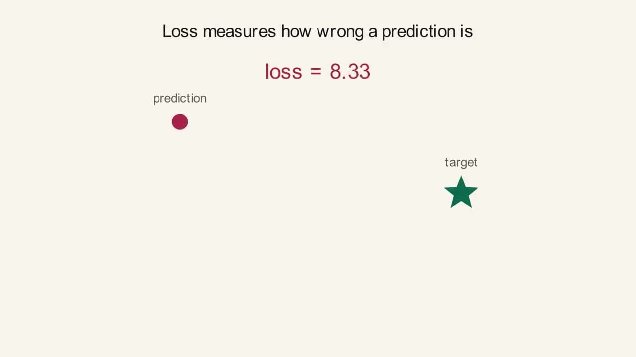
0:13What this animation shows
A red "prediction" dot sits far from a green target star while a large loss number reads 9.00 at the top of the frame. As the prediction glides toward the target, the loss number counts down and shifts from red toward green, reaching a small number as the dot lands on the target and turns green itself. This visualizes exactly what a loss function does: measure how wrong a prediction is, as a single shrinking number.
Drag the prediction toward the correct answer and watch the loss shrink toward zero.
A different loss for classification: cross-entropy
Here log always means the natural log (ln), not log base 10. Cross-entropy is defined as L = −[y·log(ŷ) + (1−y)·log(1−ŷ)]. Compare it against squared error for the same confidently wrong prediction - the network predicted ŷ=0.02 when the correct answer was y=1:
Cross-entropy scores this exact same mistake as roughly 8× worse. Why that difference matters for how a network learns, not just how it's scored, depends on backpropagation, which we haven't covered yet. We'll come back to this exact number on the output activations page, once the machinery for computing it is in place.
The network predicts 0.02 when the right answer is 1. Squared error scores that mistake at 0.4802. What does cross-entropy score it at?
- aAbout the same, near 0.5
- bRoughly double, near 1
- cRoughly eight times more, near 4
- dInfinite - it was almost completely wrong
Commit to a guess, then open this
3.9120, about eight times more. And there is no ceiling: the same prediction at 0.002 instead of 0.02 scores 6.2146, and at 0.0002 it scores 8.5172. Squared error, over that same range, only ever climbs from 0.4802 to 0.5000. One of these two losses can go on punishing a confident mistake forever and one of them cannot, and that difference is the whole page.
Everything a network learns, it learns from one number. The network makes a guess, the loss function compares that guess to the right answer, and returns a single number saying how bad the guess was. Small number, good guess. Large number, bad guess. That is the entire job.
It matters that it is one number and not a description of what went wrong. The network is never told “your answer was too high” or “you missed the cat”. It is told “0.36”, and everything else - which weight to change, in which direction, by how much - gets worked out afterwards from that single number, by the machinery the next two pages are about. Choosing a loss function is therefore choosing what the network will consider a mistake, and how strongly it will care about mistakes of different sizes. Two losses looking at the same wrong answer can disagree by a factor of eight about how wrong it was: a prediction of 0.02 when the answer was 1 scores 0.4802 under squared error and 3.9120 under cross-entropy, and both of those numbers appear below. The network trains differently as a result. This page is about those disagreements.
One piece of vocabulary before anything else, because it is used loosely everywhere else: loss usually means the score for a single example, and cost usually means the average loss over a batch of examples. Most people, including the rest of this site, use “loss” for both. Where the distinction matters below, it is spelled out.
Speeding fines
Squared error is a fine that quadruples every time you double the speed you were over by: 10 over costs a hundred, 20 over costs four hundred. MAE is a flat penalty per unit over, no matter how fast. Cross-entropy is a different court entirely: it fines you for how confidently you swore you were under the limit. Swear blind you were doing 30 in a 30 and get clocked at 60, and the fine is enormous. Say you might have been a bit over, and it is small.
Where it breaks downFines are capped by law and cross-entropy is not - it really does go to infinity.
WordsWhat one number has to carryTwo losses, in words, before either has a symbol.Rung 01
Squared error is the default loss for regression, meaning any task where the network has to produce a number rather than pick a category: a house price, a temperature, a position. You take the gap between the prediction and the right answer, and you square it.
Squaring does two things at once, and both are on purpose. It makes the score positive, so being 2 too high and 2 too low both cost the same, and it makes the cost grow faster than the mistake does. Being twice as wrong is four times as expensive. That second property is what makes squared error push hard on the worst predictions first.
Squared error is the wrong tool the moment the network’s job changes from “produce a number” to “pick a category”. For classification the network outputs a probability, a number between 0 and 1 saying how confident it is, and what you want to punish is not distance, it is misplaced confidence. Being 90% sure of the wrong answer should hurt much more than being 55% sure of the wrong answer, and it should hurt more than twice as much.
Cross-entropy does exactly that, and the mechanism is one idea: score the probability the network assigned to the answer that actually happened, and take the negative natural log of it. That is all −ln(ŷ) means. The log is there because it has one useful shape: it is 0 when the probability is 1, small when the probability is high, and it grows without limit as the probability approaches 0. There is no ceiling on the punishment for confidently ruling out the truth.
NumbersEvery loss on this page, workedSix losses, every one of them arithmetic you can check by hand.Rung 02
Here is a full trace, batch and all. The network is as small as it can be while still having something to learn: one input x, one weight w = 0.60, one bias b = 0.10, and no activation function on the output, so the prediction is just ŷ = w·x + b. The weight is positive, so it would be drawn blue on any diagram on this site. Three training examples go through it.
All three errors are negative, so the network is guessing low on every example. Look at which example the loss is mostly made of. The third one contributed 0.3600 of the 0.5400 total, two thirds of the whole score, off an error only twice the size of the other two. That is the squaring at work, and it is the reason this loss will end up caring about that example more than about the other two combined.
What happens next is that this one number, 0.0900, gets turned into a change to w and a change to b. That is not a property of squared error, it is the same procedure for every loss on this page, and it is the subject of the next page, which picks up this exact kind of network and walks the arithmetic.
That p = 0.02 row is the factor of eight from the top of this page. Squared error scores the same prediction at 0.4802; cross-entropy scores it at 3.9120, 8.15 times higher, for being confidently wrong about the same example.
Here is the full path from a raw network score to a loss, which is the part that usually gets skipped. The network’s last layer produces a raw, unbounded score called a logit, written z. Sigmoid squashes that logit into a probability. Cross-entropy scores the probability.
The third example is the interesting one. The network said 0.574, barely better than a coin flip, and got it “right” in the sense that 0.574 rounds to 1. Accuracy would score that as a win. Cross-entropy scores it as the worst of the three, worse than the example the network got wrong less confidently. Cross-entropy grades confidence, not correctness.
Now the outlier comparison. To see how far apart squared error and MAE are, compare each average against what the three well-behaved errors would have produced on their own. Three errors of 0.1 give a squared-error average of 0.01 and an MAE average of 0.1. Adding the single outlier takes those to 6.2575 and 1.325 respectively.
The two averages are not directly comparable to each other, one is in squared units and one is not, which is exactly why the comparison has to be made against each loss’s own baseline. Measured that way, one outlier out of four moves squared error roughly 47 times more than it moves MAE.
Mean absolute error itself is the plain distance between prediction and answer, |ŷ−y|. Take the same wrong prediction the demo above used, ŷ=0.02 and y=1:
That squared-error figure uses this page’s ½(ŷ−y)² convention. If you check the arithmetic yourself with the plain (ŷ−y)² form instead, you’ll land on 0.9604 for this same example, not a mistake, just a different convention.
Huber loss behaves like squared error for small mistakes and like MAE for large ones. The switch happens at a threshold you choose, δ. Worked with δ=1.0:
Huber caps how much a single outlier can dominate training, while still behaving exactly like squared error close to the target. It’s the loss behind the original DQN reinforcement-learning agent, among other places you’ll run into it.
Hinge loss, for a label y ∈ {−1, +1} and a raw score f(x), asks a coarser question than any of the above: is your raw score on the correct side of the boundary, by a comfortable margin?
PictureThe same mistake, three losses, on the number lineOne diagram, three switch positions, and the moment two losses swap places.Rung 03
Set the prediction to 0.50 with the answer at +1 in Figure 02 and read the three losses off the switch: squared error 0.1250, MAE 0.5000, Huber 0.1250. Huber and squared error agree exactly, because an error of 0.5 is inside Huber’s δ=1 threshold and Huber is squared error in there. Now drag the prediction to −1.00, an error of 2.0: squared error 2.0000, MAE 2.0000, Huber 1.5000. The two that agreed have separated, and the two that disagreed have crossed.
The red bar on the number line is the same length in every one of those readings - the bar is the error, the number underneath is what each loss thinks that error is worth.
The widget’s own static cross-entropy panel is the fourth reading the number line cannot draw: 0.480 against 3.912 for the identical prediction of 0.02. There is no bar length that shows a difference of eight times, which is exactly why that panel is separate.
EquationThe formulas, and where each symbol came fromThe same six losses as rung 2, now in symbols, with every symbol named.Rung 04
The full binary form of cross-entropy, L = −[y·ln(ŷ) + (1−y)·ln(1−ŷ)], looks like two terms but only ever uses one of them. When the true label y is 1, (1−y) is 0 and the second term vanishes, leaving −ln(ŷ). When y is 0, the first term vanishes, leaving −ln(1−ŷ). It is an if-statement written as arithmetic, which matters because the training procedure needs a loss that is differentiable, meaning it has a well-defined slope everywhere rather than jumping between two branches.
MAE’s derivative is dL/dŷ = sign(ŷ−y): always exactly +1 or −1, no matter how far off the prediction is. Every mistake, big or small, pushes the weights by the same amount. Squared error’s derivative grows with the size of the mistake instead, so a huge outlier produces a huge gradient and one bad example can dominate an entire weight update.
General caseMore than two classes, and why cross-entropy is paired with sigmoidN classes instead of two, and the one fact that decides which loss you actually use.Rung 05
With more than two categories the network produces one logit per class, softmax turns the whole set of logits into probabilities that sum to 1, and cross-entropy scores the one belonging to the correct class. Nothing about the idea changes; there are just more numbers.
Two pieces of vocabulary arrive with them. A distribution here means a list of probabilities covering every possible outcome and adding up to exactly 1, so [0.659, 0.242, 0.099] is one. And one-hot is how the correct answer gets written in the same shape: one number per class, a 1 in the position of the right answer and 0 everywhere else. “The answer is class 1, out of three” becomes [1, 0, 0].
If the true class had been class 3 instead, the same forward pass would have scored −ln(0.098566) = 2.317030 instead of 0.417030, five and a half times the loss, from identical logits. The loss depends on which answer was correct, not on how spread out the predictions were. Softmax gets its own page, Softmax for Multi-Class Output.
Now the reason cross-entropy is the standard partner for a sigmoid or softmax output, and squared error is not. The question to ask is: when the raw logit z moves a little, how much does the loss move? That quantity is written dL/dz, and for now it can be read exactly as those words - how much the loss changes when z changes - with no more machinery than that. Where such numbers come from, and what training does with them, are the next page’s subject. All that matters here is that a loss which barely moves when the network is badly wrong is a loss that will barely teach it anything.
At z = −4 the network is confidently, badly wrong: it says 1.8% for something that is true. Cross-entropy responds with −0.982, almost the largest response it can give. Squared error responds with −0.0173, 56.6 times smaller, because it multiplies the error by sigmoid’s own slope, and sigmoid’s slope is nearly zero out there. Push the logit out to −8 and the gap widens to over 2,900 times; the further into the wrong answer the network goes, the quieter squared error gets. Squared error plus sigmoid produces almost no learning signal precisely when the network is most wrong. Cross-entropy’s p − y cancels that slope term away exactly. That cancellation is the whole reason the pairing exists, and it is derived properly on the output activations page.
A precision note: p − y is the response with respect to the logit, after sigmoid has been folded in. The response with respect to the probability itself, dL/dp, is (p − y) / (p(1−p)), which does blow up near 0 and 1. Frameworks combine the sigmoid and the cross-entropy into one operation (BCEWithLogitsLoss in PyTorch) so that the clean p − y form is what actually gets computed and the unstable intermediate never appears.
The last one is not really a loss you would pick off a menu, it is a way of understanding the one you already picked. KL-divergence answers “how much worse is my predicted distribution than the true one?”, using “distribution” in the sense defined above: a list of probabilities over every outcome, adding to 1. Cross-entropy answers “how expensive is my predicted distribution?”, and part of that expense is unavoidable: even a perfect prediction costs something, because the true distribution has its own built-in uncertainty. KL-divergence is cross-entropy with that unavoidable part subtracted off, so a perfect prediction scores exactly 0.
Cross-entropy decomposes as H(P,Q) = H(P) + D_KL(P‖Q), so minimizing cross-entropy and minimizing KL-divergence are the same optimization problem in practice - H(P), the true data’s own uncertainty, doesn’t depend on the model at all. Quick worked check: true distribution P=[0.7, 0.3], predicted Q=[0.5, 0.5] gives H(P)=0.610864 and H(P,Q)=−ln(0.5)=0.693147, so D_KL=0.082283, matching a direct KL calculation, 0.7×ln(1.4) + 0.3×ln(0.6) = 0.082283. You’ll see this term again if you go on to study generative models.
Six losses is a lot to hold at once. The choice is usually made by the shape of the output, not by taste:
If you are unsure, the shape of your output layer has already decided for you. That is not a coincidence; the page on output activations is the other half of this one.
Why this and not that
Why not just train on accuracy? That is what I actually care about.
Accuracy is a count, and counts do not have slopes. Move a prediction from 0.51 to 0.62 and the accuracy is identical, so there is nothing to tell the network which way to move next. Every loss on this page is chosen partly because it changes smoothly when the prediction changes slightly. Accuracy is what you report; the loss is what you train.
Why square the error rather than take the absolute value? Squaring feels arbitrary.
Two reasons, and one of them is not the one usually given. It makes the cost grow faster than the mistake, which is a real design choice, and it also makes the loss smooth at zero, where the absolute value has a corner. MAE’s slope is +1 on one side of the answer and −1 on the other and never anything in between, which is why it never settles down close to the target.
Why the natural log and not log base 10?
Base 10 works identically; every value is just divided by ln(10) = 2.302585, a constant, so it rescales every score without changing which prediction scores best. The natural log is the convention because its slope is exactly 1/p, with no constant hanging off it, which keeps the derivative clean.
Is cross-entropy just a fancier squared error?
No, and the dL/dz block in rung 5 is the reason. When the network is confidently wrong, squared error’s push on the raw score is 56.6 times weaker than cross-entropy’s, and past z = −8 it is over 2,900 times weaker. They are not the same loss with different constants; one of them stops teaching precisely when the network most needs teaching.
The page says ‘loss’ and my textbook says ‘cost’ and ‘objective’ and ‘criterion’.
Loss is normally one example, cost is normally the batch average, objective is whatever you are optimising including any regularization terms, and criterion is PyTorch’s variable name for the loss object. In practice everyone says loss for all four, including the rest of this site.
- Entropy
- Borrowed from thermodynamics, where Clausius coined it in 1865 for the unusable part of a system’s energy. Shannon reused it in 1948 for the average surprise in a stream of messages, which is the sense every use on this page has.
- Cross-
- In cross-entropy: you are scoring one distribution using the code that would have been optimal for a different one. Your predictions are the code, the truth is the data, and the cross is where the two meet.
- Hinge
- The graph of max(0, 1 − y·f(x)) is a straight slope that stops dead at zero and stays flat. It looks like a hinge, and the flat part is where the loss no longer cares.
- Huber
- Peter Huber, the Swiss statistician who published it in 1964 in a paper about making estimates that survive contaminated data. It was designed for outliers before neural networks existed.
- KL
- Solomon Kullback and Richard Leibler, 1951. Their own word for it was “divergence” rather than “distance”, deliberately, because it is not symmetric: D(P‖Q) and D(Q‖P) are different numbers.
- MSE, MAE
- Mean squared error, mean absolute error. The only difference in the names is the only difference in the formulas.
- What is happening
Squared error is bounded on this interval: the very worst it can say about a prediction is 2.0000, and it is already saying 1.9013. Being slightly more wrong barely changes the number, so the push toward being right barely changes either. The widget’s own cross-entropy panel scores a comparable mistake at 3.912 and would keep climbing forever.
- Fix
Sigmoid output and binary cross-entropy, or softmax output and categorical cross-entropy. Frameworks combine the two into one call for numerical reasons -
BCEWithLogitsLoss,CrossEntropyLoss.- Watch for
- Drag from −0.95 to −1.00. The loss moves from 1.9013 to 2.0000 and then stops, because it has hit its own ceiling.
- What is happening
0.05 with an answer of +1 is on the correct side of zero, so any accuracy metric scores this as a win. The loss scores it 0.4513, three and a half times worse than a prediction of 0.50 would score. Loss grades how far and how confidently; accuracy grades which side of a line you landed on. They can move in opposite directions for a whole epoch.
- Fix
Track both. Use the loss to train and to early-stop, and the accuracy to talk to people about.
- Watch for
- Sign is right, score is bad. Both readings are correct and they are answering different questions.
- What is happening
The widget prints 0.500, and by hand you would get
(0 − 1)² = 1.000. Neither is wrong. This site uses the ½ convention throughout, because the ½ cancels the 2 that appears when the loss is differentiated and every gradient on the next four pages comes out cleaner for it. A loss that is exactly double someone else’s is the single most common “my numbers do not match the tutorial” bug.- Fix
Check for the ½ before comparing any two sources’ loss values. A factor of exactly 2 is almost never a real disagreement.
- Watch for
- 0.500 on screen where your arithmetic said 1.000.
- What is happening
Drag from 0.90 to 0.95 to 1.00 and the MAE readout falls 0.1000 → 0.0500 → 0.0000, in equal steps. Equal steps mean a constant slope, which means MAE pushes just as hard when the prediction is 0.99 as when it is 0.5. Squared error, over the same drag, falls 0.0050 → 0.0013 → 0.0000, easing off as it arrives. MAE never eases off, so with a fixed learning rate it steps over the answer and back forever.
- Fix
Huber. It is squared error inside δ and MAE outside it, so you get the outlier resistance without the jitter at the target.
- Watch for
- Three equal drops for MAE against three shrinking drops for squared error, on the identical drag.
- What is happening
At an error of 0.5, Huber reads 0.1250, identical to squared error’s 0.1250 and nothing like MAE’s 0.5000. At an error of 2.0, Huber reads 1.5000, below squared error’s 2.0000 and below MAE’s 2.0000. It is not a compromise between the two on every example, it is exactly one of them on every example, and δ decides which.
- Fix
Choose δ deliberately. It is the error size at which you stop believing the example and start capping it, so it belongs in the same units as your target.
- Watch for
- The Huber and squared readouts printing the identical 0.1250, then separating the moment the error crosses 1.0.
Drag the prediction toward the correct answer and watch the loss shrink toward zero.
A different loss for classification: cross-entropy
Here log always means the natural log (ln), not log base 10. Cross-entropy is defined as L = −[y·log(ŷ) + (1−y)·log(1−ŷ)]. Compare it against squared error for the same confidently wrong prediction - the network predicted ŷ=0.02 when the correct answer was y=1:
Cross-entropy scores this exact same mistake as roughly 8× worse. Why that difference matters for how a network learns, not just how it's scored, depends on backpropagation, which we haven't covered yet. We'll come back to this exact number on the output activations page, once the machinery for computing it is in place.
- 01Get the squared-error readout to exactly 0.0000 twice, using two different target settings.
Hint
The loss is zero only when the prediction equals the answer, and the answer can be either +1 or −1.
Answer
Prediction +1.00 with target +1, and prediction −1.00 with target −1. Both ends of the slider are reachable. The point is that zero loss is not a property of the prediction, it is a property of the pair.
- 02Find a prediction where squared error and MAE give the same number, and say why that particular value.
Hint
Squared error here is
0.5·e²and MAE is|e|. Set them equal.Answer
0.5·e² = |e|when|e| = 2, so prediction −1.00 with target +1: both read 2.0000. Below an error of 2 the ½ makes squared error the smaller of the two; above it, squared error would be larger. On this slider, 2.0 is the largest error available, which is why the two curves meet exactly at the end of the track and nowhere else. - 03With the answer at +1, find the prediction where Huber stops agreeing with squared error, to the nearest 0.05.
Hint
Huber’s two branches swap at
|e| = δ, and this widget’s δ is 1.0.Answer
Prediction 0.00, where the error is exactly 1.0 and both read 0.5000. At prediction 0.05 (error 0.95) they still agree at 0.4513. At prediction −0.05 (error 1.05) squared error reads 0.5513 and Huber reads 0.5500, and from there they separate for good. The gap widens with every further step, which is the whole design.
- 04Predict, before dragging: as the prediction moves from 0.00 to −1.00, does the gap between squared error and Huber grow steadily, or accelerate? Check it.
Hint
Write down the three readings at 0.00, −0.50 and −1.00 for both losses and take the differences.
Answer
It accelerates. Squared 0.5000 / 1.1250 / 2.0000 against Huber 0.5000 / 1.0000 / 1.5000, so the gaps are 0.0000, 0.1250, 0.5000. The gap quadruples over the second half of the drag. That is squared error’s quadratic growth pulling away from Huber’s linear branch, and it is precisely how much influence one outlier is buying itself.
- 05Using only the widget’s static cross-entropy panel and the switch, argue that the loss you pick changes which example the network works hardest on.
Hint
Compare the ratio between two examples’ scores, not the scores themselves.
Answer
Take an error of 0.5 and an error of 2.0. Under MAE they score 0.5000 and 2.0000, a ratio of 4. Under squared error, 0.1250 and 2.0000, a ratio of 16. Under the panel’s cross-entropy, a prediction of 0.02 against 1 scores 3.912 while squared error scores 0.480, a ratio of 8.15 for the same single example. The bad example is worth four times more under squared error than under MAE, and the confidently wrong example is worth eight times more under cross-entropy than under squared error. The loss is a weighting over your dataset, and you chose it.
- PyTorch
nn.CrossEntropyLossis one line, and it is the line that trains almost every image classifier you have ever used. It takes raw logits, not probabilities, precisely because of thep − ycancellation in rung 5. - DeepMind’s DQNThe 2015 Atari agent used Huber loss rather than squared error, for the reason on this page: a single freak reward would otherwise have produced a gradient large enough to wreck the network.
Squared error asks how far the arrow landed from the gold. Cross-entropy asks how much you bet before you shot.
Which question you ask decides which mistakes your network works hardest to never make again.
A loss is a single number saying how bad a guess was. It says nothing about which of the network’s thousands of weights was responsible, or which way to move any of them. Nothing on this page can turn 0.0900 into a change to w. That conversion is a separate machine, and building it takes the next two pages: one to define what “which way to move” even means, and one to compute it for every weight at once.