Optimizers
How optimizers like momentum, RMSProp, and Adam improve on plain gradient descent.
Same landscape, same learning rate, six clicks apart
Three optimizers, one landscape, one starting point, one learning rate. Six clicks.
One of them is nine times worse than where it started. Nothing about the problem changed between those two rows - only what each one does with the gradient after it receives it.
Before this page - 2 pages needed, 1 borrowed from later3
Gradients and Gradient Descent
every optimizer here takes a gradient as input and produces a weight change; this page only ever changes what happens in betweenLoss Functions
the gradient being passed around is the gradient of a loss, and which loss decides how large it isRegularization
AdamW is a fix to weight decay, and weight decay and lambda are defined three pages after this one. Both are given a short primer in rung 4, on loan.comes later
Leave the learning rate where it is. Press ‘Take a step’ five times and watch which ball is closest to the bottom. Then guess which one will still be closest after twenty.
 0:14
0:14What this animation shows
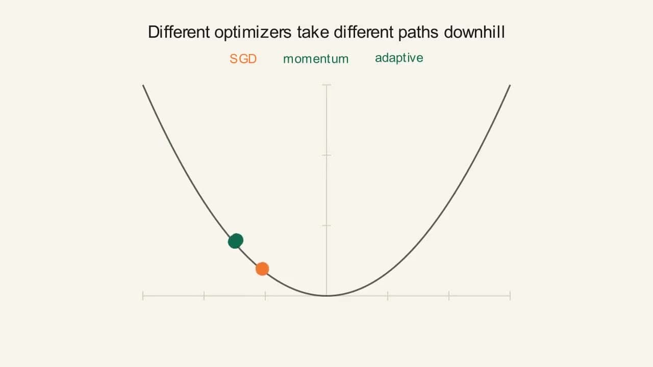
Three colored balls, labeled SGD, momentum, and adaptive, start together at the same point on a parabola and move downhill along visibly different paths at different speeds. The plain SGD ball takes small, even steps; the momentum ball swings through with more built-up speed; the adaptive ball adjusts its stride as it goes. This previews the page's core idea: optimizers built on top of plain gradient descent reach the minimum in different, often faster, ways.
All three start at x=2.4 on the same landscape and step together, so distance from the bottom after the same number of steps is a direct comparison.
Toggle optimizers, pick a shared learning rate, then take steps and watch how far each ball travels per step and how it settles near the bottom.
After five steps at lr = 0.1 on this bowl, which of the three is nearest the bottom?
- aAdam - it is the modern one everyone uses
- bMomentum - it accumulates speed
- cPlain gradient descent - it has no tricks at all
- dThey are all about the same
Commit to a guess, then open this
Plain gradient descent, at x = 0.786. Momentum is at −1.393, having overshot the bottom two steps ago. Adam is at 1.902, barely a fifth of the way there. Adam is last, and that is not a bug and not a bad implementation: Adam deliberately normalises its step to about ±lr regardless of how steep the ground is, so its first step is 0.100 while plain gradient descent’s is 0.480. On a single smooth bowl, throwing away the size of the gradient is throwing away good information. Rung 5 builds the landscape where throwing it away is the right call, with numbers.
The gradient descent you just learned computes an exact average gradient over your entire dataset before taking one step - accurate, but potentially slow at scale. It’s also just the simplest member of a much larger family of ways to use a gradient once you have one.
Every optimizer below takes the same input, a gradient, and produces the same kind of output, a change to the weights. What differs is only how much of the past each one remembers and what it does with that memory. To make the differences mechanically visible rather than described, every section on this page runs the same problem from the same starting point: the bowl f(x) = x², starting at x=2.4, with lr=0.1 throughout. The gradient at any point is 2x, and the bottom is at x=0.
Before any of the clever ones, the plain one. Stochastic gradient descent exists for a reason that has nothing to do with mathematics: computing the exact gradient means running every training example through the network before you are allowed to change a single weight. On a dataset of a million images that is a million forward passes for one update. SGD’s answer is to stop insisting on the exact gradient and accept a rough one computed from a handful of examples, on the grounds that a hundred rough steps beat one perfect step. Everything else on this page assumes you have already made that trade, and asks what to do with the rough gradients once you have them.
A car on a winding road
Plain gradient descent is steering by where the road points at this exact instant, correcting hard at every bend, which is how you get a passenger sick. Momentum is a heavy car: it holds its line through a wobble in the road surface, which is what you want, and it also runs wide on a tight corner, which is what overshoot is. Nesterov is looking at the corner rather than feeling it, so it starts braking a moment earlier. The rows in rung 2 show that earlier braking: after five steps momentum has overshot to −1.393 and Nesterov to only −0.624.
Where it breaks downA car has one direction of travel. A network is steering in a million directions at once and they disagree.
WordsSeven ways to use one gradientWhat each optimizer remembers, in one sentence each, before any symbols.Rung 01
Every optimizer takes the same input, a gradient, and produces the same kind of output, a change to the weights. What differs is only how much of the past each one remembers and what it does with that memory.
Momentum. Plain gradient descent’s “ball” has no memory - every step is decided purely by the current slope, so on a landscape shaped like a narrow valley it can zig-zag across the valley walls instead of smoothly rolling toward the far end. Momentum gives the ball velocity that accumulates: it remembers recent downhill directions and keeps drifting that way even where the current slope briefly disagrees, canceling the zig-zag and speeding up consistent progress.
Nesterov. Momentum computes the gradient where it currently stands, then adds the accumulated velocity and moves. But the velocity is going to carry it somewhere regardless, so the gradient it just measured is already slightly out of date by the time the move happens. Nesterov momentum measures the gradient at the place the velocity is about to take it, and uses that instead. It is the difference between braking when you feel the wall and braking when you see it.
AdaGrad. Momentum fixes direction. AdaGrad instead fixes the fact that one single global learning rate is wrong for every parameter simultaneously - some parameters (rarely-updated ones) need larger steps, others need smaller ones. AdaGrad tracks how much each parameter has moved historically and shrinks its personal step size the more it’s already moved. The known flaw: that running sum only ever grows, so the step size keeps shrinking and eventually grinds to a near-halt even if the model still has more to learn.
RMSProp. AdaGrad’s own fix for AdaGrad: keep the idea of a personal step size per parameter, but replace the ever-growing sum with a decaying running average, so old gradient history fades out and the step size can recover instead of only ever shrinking.
Adam. Combines momentum’s idea (track a running average of the gradient itself, for direction) with RMSProp’s idea (track a running average of the squared gradient, for a safe adaptive step size), plus one correction neither of those needs on its own: since both running averages start at zero, they’re artificially biased toward zero for the first few steps, so Adam explicitly corrects for that bias.
AdamW. One more refinement: naively adding L2 weight decay to Adam, by folding it into the gradient before Adam’s adaptive rescaling, means that rescaling ends up distorting the decay too, applying it unevenly per parameter. AdamW’s fix is to apply weight decay directly to the weights, completely separate from the adaptive gradient step.
NumbersAll seven, same start, five stepsOne table with all seven rows, then every row derived, step by step.Rung 02
Plain gradient descent wins this race, and it is worth saying plainly why rather than hiding it. Its step size is proportional to the gradient, and at x=2.4 the gradient is 4.8, so its first step is a large 0.48. Adam deliberately normalises its step to roughly ±lr regardless of gradient size, so its first step is exactly 0.1. On a single smooth bowl where the gradient is helpfully large, throwing that information away is a loss. Rung 5 shows the landscape where throwing it away is a win, with numbers.
Momentum and Nesterov overshoot past the bottom entirely by step 4, which is not a bug; that is what accumulated velocity does, and it is the price of the speed that gets them there in three steps instead of five.
Six blocks follow, each deriving one row of the table above by hand. They build on each other in pairs - momentum then Nesterov (both remember direction), AdaGrad then RMSProp (both scale the step per parameter), then Adam and AdamW (which combine the two ideas). Worth reading once in order; after that, each block stands alone as a reference.
Momentum, derived. Same x² landscape and starting point, x₀=2.4, lr=0.1, β=0.9:
Nesterov, derived in the same convention, so the two are directly comparable. The only change from plain momentum is where the gradient is evaluated: at the peeked-ahead position rather than the current one.
Step 4 is where the lookahead earns its keep. Plain momentum’s rule, applied standing where Nesterov now is at x=0.427008, would measure a gradient of +0.854016 and keep accelerating downhill. Nesterov peeks to x=−0.260045, discovers the gradient has already flipped to −0.520090, and starts braking a full step earlier. (Plain momentum, running its own race from the start, is at 0.148800 after three steps, which is why that number and not 0.427008 appears in its row of the comparison table; the comparison here is between the two rules evaluated at the same place.) The result is visible in the table: after 5 steps momentum has overshot to −1.393008 while Nesterov is at −0.623660, less than half as far past the bottom.
Momentum and Nesterov both still take a step whose size depends only on the learning rate and the accumulated velocity - every parameter is treated the same way. AdaGrad tries a different idea entirely: give each parameter its own step size, shrinking it for parameters whose gradient has historically been large.
AdaGrad, derived.
AdaGrad’s per-parameter shrinking never lets up, even once a parameter’s gradients calm down, since it keeps adding every squared gradient it has ever seen. RMSProp keeps the same per-parameter idea but forgets old gradients over time instead of piling them up forever.
RMSProp, derived.
Unlike AdaGrad, this doesn’t shrink forever - since s is a decaying average, it settles at a fixed point under a constant gradient, the exact fix RMSProp promised over AdaGrad’s permanent shrink.
Two ideas have now been built separately: momentum’s running direction, and AdaGrad/RMSProp’s per-parameter step-scaling. Adam is what happens when a single optimizer tracks both at once, plus one extra fix for the first few steps, when both running averages start at zero and are biased low.
Adam, derived, x₀=2.4, lr=0.1, same landscape:
This isn’t a coincidence: at t=1, the bias correction perfectly cancels the running-average weighting for ANY gradient value, so Adam’s very first step always moves by exactly ±lr, regardless of how large the raw gradient was.
AdamW, derived. The claim that folding L2 decay into Adam’s gradient lets Adam’s rescaling distort the decay is checkable. Adam divides every update by √ŝ, and √ŝ tracks the size of that parameter’s own recent gradients. So a decay term that got folded into the gradient gets divided by the parameter’s gradient size too. Take two weights in the same network, both at w = 0.5, both with λ = 0.1 and lr = 0.1. Weight A sits in a busy part of the network with a steady gradient of 2.0. Weight B is in a quiet part, gradient 0.002.
One λ was requested and, under Adam with L2, thirty-nine different strengths of decay were delivered, purely as a side effect of which weights happen to have large gradients. AdamW’s decay term sits outside the m̂/√ŝ fraction entirely, so it does exactly what it says regardless of gradient size.
Two things flagged as exaggerated or simplified. λ = 0.1 is far larger than anything you would train with; realistic values run from about 0.01 down to 0.0001, and 0.1 is used here only so the distortion is legible at eight decimal places instead of buried at twelve. And √ŝ ≈ |g| is an approximation that holds when a parameter’s gradient is roughly steady. During real training gradients move around and the exact ratio moves with them, but the direction of the distortion - big-gradient parameters get less decay than you asked for and small-gradient parameters get more - is not an approximation.
And the batch trade-off, in numbers. Four data points, targets=[1.8, 2.2, 1.9, 6.0], current weight w=2, using the gradient formula 2×(w−target) per point. Individual per-point gradients: [0.4, −0.4, 0.2, −8.0]. The full-batch average is −1.95. A single-example SGD step might draw gradient +0.4 or −8.0 depending on which point gets picked, wildly different directions from the exact same starting weight. A mini-batch of 2 (say, points 3 and 4) averages to −3.9, closer to the true full-batch gradient than any single point alone, though still not exact. As batch size grows toward the full dataset, the estimate’s noise shrinks toward the true gradient.
PictureThree balls, one landscapeWhat each row of the table looks like as motion, and how to read the trail.Rung 03
The three balls in Figure 02 are rows 1, 2 and 6 of that table, drawn. Press ‘Take a step’ three times with all three shown. Plain GD’s dots are evenly spaced and shrinking - each one is 80% of the last distance from the bottom. Momentum’s dots get further apart each time, which is velocity accumulating, and by step 4 it has crossed the bottom and its dots are on the other side. Adam’s dots are almost equally spaced and tiny, because Adam’s step is pinned near ±lr no matter how steep the ground is: at step 1 the gradient is 4.8 and Adam still moves exactly 0.1.
The fading trail is five steps long, so once a ball has settled the trail collapses into a single dot, and once a ball has diverged the trail runs off the frame and the ball sticks to it - at which point the numbers underneath are the only honest reading.
EquationEvery update rule, in one conventionSeven update rules, one convention, so they can be compared line by line.Rung 04
Two words first, because AdamW is built on them and they properly belong to a later page. Weight decay is a second pull applied to every weight on every step, always toward zero, on top of whatever the gradient asked for. It exists because large weights are what an overfitted network is made of, so shrinking them a little on every step is a cheap way to keep the network from memorising its training data. Its strength is a single number, λ (lambda): at λ = 0 there is no pull at all, and the larger λ gets, the harder every weight is dragged toward zero.
That is everything you need to read the AdamW line below. Why you would want it, what it does to a network’s behaviour, and the difference between the two ways of writing it down are the regularization page’s subject.
Every line above is written in one convention: v accumulates raw gradients and the learning rate is applied outside it. Papers vary, and the same letter v in another source may already have the learning rate and the minus sign folded into it. If two sources’ numbers will not reconcile, check that before checking the arithmetic.
The decay term in AdamW, on the right, is untouched by anything Adam is doing to the gradient. This is why “Adam with weight_decay=0.01” in most modern frameworks actually means AdamW under the hood.
General caseThe landscape where the adaptive ones winTwo dimensions instead of one, and the result inverts.Rung 05
The comparison table near the top of this ladder shows plain gradient descent beating every adaptive method. That result is real, and it is a property of the landscape, not of the optimizers. A single symmetric bowl is the best possible case for a single global learning rate, because one step size genuinely suits every direction.
Real loss landscapes are not symmetric. Change one thing about the test problem, make it two-dimensional with one direction twenty times steeper than the other, f(x, y) = ½(x² + 20y²), start at (5.0, 1.0), and the picture inverts.
That is the zig-zag the momentum section described in words, now written out as numbers. And it explains the real constraint, which is not “gradient descent is slow” but “gradient descent’s learning rate is set by its steepest direction and then every other direction has to live with that choice”. The multiplier for y stays inside (−1, 1) only while lr < 2/20 = 0.1. Push lr to 0.11 and y’s multiplier is −1.2 and the run diverges, even though the x direction would have been perfectly stable up to lr = 2. One direction is holding the whole run hostage, twenty times below the rate the other direction wants.
RMSProp and Adam divide each direction by the size of its own recent gradients, which decouples the two: y no longer sets x’s speed limit. On this small example that decoupling costs more than it saves over eight steps, because the shallow direction still only moves at lr per step. In a real network with millions of parameters and gradient magnitudes spanning several orders of magnitude, the decoupling is the whole ballgame, and it is why Adam is the default that most training runs start from.
Flagged as simplified: two parameters standing in for millions, and a quadratic bowl standing in for a loss surface that is not quadratic anywhere. The mechanism, per-direction step sizes versus one shared step size, is exactly the real one.
One more knob, separate from all of the above: every optimizer on this page still takes a learning rate lr as an input - none of them decide it for you. In practice, that learning rate is rarely held perfectly constant for the whole training run: a common pattern is a short warmup (starting small and ramping up, so the first few updates, before the running averages inside Adam/RMSProp have gathered enough history to be reliable, don’t take an oversized step) followed by decay (gradually shrinking the learning rate as training progresses, so later updates fine-tune instead of overshoot). That’s a schedule on top of whichever optimizer you pick - Adam with a decaying learning rate is still Adam, just with one more moving part layered on.
Why this and not that
If Adam loses this race, why does everyone use it?
Because this race is a symmetric one-dimensional bowl, which is the single best case for one shared learning rate and the single worst case for adaptivity. Rung 5 changes exactly one thing - makes one direction twenty times steeper than the other - and plain gradient descent’s learning rate becomes hostage to the steep direction while every shallow direction crawls. Real networks have millions of directions and gradient magnitudes spanning orders of magnitude.
Should I use momentum or Adam? Adam already has momentum in it.
Adam’s m is a running average of the gradient, which is momentum, so “Adam plus momentum” is not a thing. The real choice is Adam/AdamW versus SGD-with-momentum, and it is genuinely contested: Adam converges faster and more reliably without tuning, while carefully tuned SGD-with-momentum still wins some vision benchmarks on final accuracy. Start with AdamW.
Why does AdaGrad exist if RMSProp fixes it?
AdaGrad is the idea; RMSProp is the patch. Knowing the flaw is what makes RMSProp’s decaying average obviously necessary rather than an arbitrary extra γ. AdaGrad is also still genuinely used where the permanent shrink is a feature, on very sparse problems where a rarely-seen parameter should keep its large step size for a long time.
What is bias correction actually correcting?
Both of Adam’s running averages start at exactly zero, so on step 1 the average of the gradient is 90% zero and 10% real gradient - an estimate ten times too small, purely from the starting value. Dividing by (1 − β₁ᵗ) removes exactly that artefact. Its effect vanishes as t grows, which is why it only matters for the first few dozen steps and why it matters enormously there.
Is the learning rate still my problem if I use Adam?
Yes. Every optimizer on this page takes lr as an input and none of them decides it. Adam narrows the range of values that work, which is most of why it is popular, but the reference case at the top of this page is Adam’s own landscape at lr = 1.10, and the run still falls apart.
- Stochastic
- Greek stokhastikos, “able to guess”. The gradient from one random example is a guess at the true gradient, right on average and wrong on any given step.
- Momentum
- Straight from physics: mass times velocity, the property that keeps a moving thing moving. The analogy is exact enough that the update is often derived as a ball rolling with friction, where β is how little friction there is.
- Nesterov
- Yurii Nesterov, who published the accelerated-gradient method in 1983, thirty years before anyone applied it to a neural network.
- Ada-
- In AdaGrad and Adam, short for adaptive: the step size adapts per parameter instead of being one shared number.
- RMS
- Root mean square. Square the gradients, take their mean, take the square root: the name is the formula, read backwards.
- Adam
- Not a person. It stands for ADAptive Moment estimation, the “moments” being the running average of the gradient (first moment) and of the squared gradient (second moment).
- W
- In AdamW, for the decoupled Weight decay that the paper’s title is about. The whole contribution is moving one term outside one fraction.
- What is happening
On this bowl plain gradient descent’s step is
x ← x·(1 − 2·lr). At lr = 1.10 the multiplier is −1.20: every step crosses the bottom and lands 20% further out than it started. Six steps take the loss from 5.7600 to 51.3567, and the growth is geometric, so it never comes back. Adam is shown alongside precisely because it does not diverge here - its step is capped near ±lr by construction, so at the same catastrophic learning rate it is merely wandering, at loss 1.6591.- Fix
Cut the learning rate by a factor of ten and re-run. This is the first thing to try, before the architecture, the data, or the initialisation.
- Watch for
- The plain ball is pinned against the right-hand edge of the chart from step 3 - it has run off the end of the frame. Read the numbers underneath instead: x = 7.1664, loss = 51.3567, and both are still growing.
- What is happening
Adam has moved 0.299 in six steps, from 2.400 to 2.101. It is doing exactly what it is designed to do: step by about ±lr per step regardless of gradient size, and lr is 0.05. Six steps is 0.3. There is no bug here and there is nothing to fix in the code.
- Fix
Judge an optimizer over hundreds of steps, not six, and remember that Adam’s step size is set by lr almost alone. If Adam is slow, the learning rate is the knob, not the optimizer.
- Watch for
- Adam’s five trail dots almost evenly spaced and almost touching - equal-sized steps are Adam’s signature, and here they are equally small.
- What is happening
At lr = 0.50 plain gradient descent lands exactly on the bottom in one step and stays there. Momentum, from the identical start, overshoots to −2.16, comes back past the bottom, and after six steps is at 1.557 with a loss of 2.42. Accumulated velocity is not a free improvement: it is stored energy, and on a landscape where the plain step was already right, the stored energy has nowhere to go but past the target.
- Fix
Momentum’s β and the learning rate have to be tuned together. Raising β without lowering lr is raising the effective step size, often by a lot: at β = 0.9 the steady-state step is roughly ten times the plain one.
- Watch for
- The plain ball sitting motionless at the bottom for six consecutive clicks while the momentum ball crosses the screen twice.
- What is happening
Adam is last, at more than twice plain gradient descent’s distance from the bottom. Plain GD’s first step is 0.480 because the gradient there is 4.8 and it uses that number. Adam’s first step is exactly 0.100 because at t = 1 the bias correction cancels the running-average weighting exactly, for any gradient whatsoever. Adam threw away a useful number on purpose, and on this landscape that number was worth having.
- Fix
Nothing to fix here. Recognise the shape of the problem: adaptivity pays where gradient magnitudes differ wildly between parameters, and costs where they do not.
- Watch for
- The three balls in reverse order of reputation, and Adam’s trail being visibly the most evenly spaced of the three.
- What is happening
Momentum’s loss falls to 0.0221 at step 3, then rises to 0.5485, 1.9405, 2.8952 - three consecutive steps of the loss getting worse. That looks exactly like the divergence in M1 and it is not: keep clicking and it reads 2.6860, 1.5744, 0.4331, then 0.0001 at step ten. It was a single overshoot decaying, not a runaway. The two are told apart by whether each swing is larger or smaller than the last, never by whether the current step was worse than the previous one.
- Fix
Before cutting a learning rate because the loss rose, check whether the amplitude is growing or shrinking. Momentum runs are supposed to overshoot; that is what buys the speed.
- Watch for
- The loss rising for three steps in a row and then coming back to 0.0001 by step ten, without changing anything.
All three start at x=2.4 on the same landscape and step together, so distance from the bottom after the same number of steps is a direct comparison.
Toggle optimizers, pick a shared learning rate, then take steps and watch how far each ball travels per step and how it settles near the bottom.
- 01Reproduce the first row of the seven-way table exactly: plain gradient descent at lr = 0.1, five steps.
Hint
Take the steps one at a time and read the number after each.
Answer
1.9200, 1.5360, 1.2288, 0.9830, 0.7864 - the table’s Plain GD row, to four decimals. Each is 0.8 times the last, because the multiplier
(1 − 2·lr)is 0.80 and never changes on this landscape. - 02Find, to two decimals, the largest learning rate at which plain gradient descent still converges, and confirm Adam does not diverge at any value the slider allows.
Hint
The multiplier
(1 − 2·lr)has to stay inside −1 and +1.Answer
lr = 0.99 converges (multiplier −0.98, each swing keeping 98% of the last); lr = 1.00 bounces between ±2.4 forever; anything above diverges. Adam never diverges at any slider value up to 1.10, because its update is
lr·m̂/(√ŝ+ε)and that fraction is close to ±1 whatever the gradient is - so its step is bounded by roughly lr, and a bounded step on a bowl of this size cannot run away. That bound is Adam’s real selling point and it is visible right here. - 03Get momentum to arrive at the bottom and stay there, without lowering the learning rate below 0.10.
Hint
You cannot change β in this widget. So the question is not how to stop the overshoot, it is how many steps the overshoot takes to die.
Answer
You wait. At lr = 0.10 momentum reaches 0.1488 at step 3, overshoots to −1.7015 by step 6, and is back at 0.0106 by step 10, having crossed the bottom twice. The oscillation decays because β = 0.9 loses 10% of the stored velocity every step. The honest answer to this task is that momentum trades a guaranteed overshoot for arriving much sooner - at step 3 it was already closer than plain GD ever got in five - and the overshoot is the price, not a fault.
- 04Set up the divergence case yourself, then find the smallest slider value at which plain GD’s loss is higher after six steps than it was at the start.
Hint
Six steps of multiplier
mleaves the weight at2.4·m⁶. When is that bigger than 2.4?Answer
Any lr above 1.00 - at lr = 1.01 the multiplier is −1.02 and
1.02⁶ = 1.126, so after six steps the loss is 1.27× its starting value, a rise slow enough to look like noise. At the slider’s maximum of 1.10 the same six steps give1.2⁶ = 2.986, a weight of 7.166 and a loss of 51.357, 8.9× the start. Divergence does not announce itself; at lr = 1.01 it takes about seventy steps to become obvious, and it was already unrecoverable at step one. - 05Using nothing but this widget, explain why the seven-way table’s Adam row moves by almost exactly 0.0999 every step after the first.
Hint
Look at what
m̂/√ŝis when the gradient has been roughly the same size for several steps.Answer
When the gradient is steady,
m̂is approximatelygand√ŝis approximately|g|, so the fraction is approximately ±1 and the step is approximately ±lr = 0.1. The table’s row confirms it: 2.400 → 2.300 → 2.200134 → 2.100498 → 2.001197 → 1.902341, each step within 0.0002 of 0.1. Adam has, deliberately, thrown away all information about how steep the ground is, and kept only the sign. On this bowl that is a loss; in rung 5’s valley it is what stops the steep direction from setting the speed limit for the shallow one.
- GPT-3Was trained with Adam using beta1 = 0.9, beta2 = 0.95, epsilon = 1e-8 and weight decay 0.1, with a warmup then cosine decay on the learning rate - which is the closing paragraph of rung 5, at scale.
- The Adam paperKingma and Ba, 2014, is one of the most-cited papers in the whole of science, with well over a hundred thousand citations. Almost every model you have used was trained by the eight lines in rung 4.
Plain gradient descent feels the ground. Momentum remembers where it was already going. Adam gives every weight its own private stride.
Which of the three wins is a fact about the landscape, never about the optimizer.
Every optimizer on this page takes a gradient and improves what happens after it arrives. None of them can do anything about a network whose gradients were doomed before the first step was taken. A layer whose weights all started identical produces identical gradients forever, and no amount of momentum or per-parameter scaling separates two numbers that are equal. A layer whose weights started at the wrong scale saturates its activations on the first forward pass, and a saturated tanh has a slope of zero, which every optimizer here faithfully multiplies by its learning rate to get zero. The next two pages are about the numbers you have to get right before any of this machinery is allowed to run.