Backpropagation
The chain rule in action: a full worked forward and backward pass, weight by weight.
One number, nine questions
One network, nine weights, one wrong answer. Here is the size of the problem.
Guessing is not an option: a real network has millions of these and they interact. Trying each one in turn is not an option either; that is millions of forward passes for one step. There is exactly one procedure that answers all nine questions at once, in a single backward sweep costing about as much as one forward pass, and this page is that procedure, performed by hand.
Before this page - 4 pages, and this is the one that pays them all back4
Two earlier pages borrowed a definition from this one. If you met δ on the weight initialization page or “the gradient arriving at y” on the training-time regularization page, this is where both are actually derived.
Gradients and Gradient Descent
dL/dw, the nudge-and-measure definition of a slope, and the update rule this page’s last stage appliesLoss Functions
the half-squared-error convention, which is why the first backward step is (o_out − y) with no stray factor of 2Activation Functions
the closed-form slope formulas 1 − tanh²(x) and s(1−s), which this page multiplies by at every layerLayers and the Forward Pass
the forward pass this page runs before it can run anything backward
Press ‘Next step’ twelve times and read each line as it appears. Do not try to hold the whole thing at once; each stage is one multiplication, and the highlighted neuron on the diagram tells you where you are.
 0:16
0:16What this animation shows
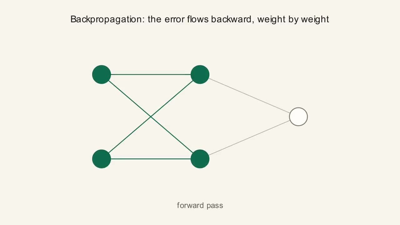
A small network (two inputs, two hidden neurons, one output) first lights up left to right in a forward pass, ending at a red "loss" dot beside the output. The caption switches to "backward pass: gradients flow right to left," and a red pulse travels back through the network, layer by layer, each neuron briefly flashing as it receives its share of the error. This is backpropagation: working backward from the loss, through the chain rule, to find which direction to nudge every weight.
Step 1 of 12: Forward pass - h1's weighted sum
inputs: x₁ = 0.50, x₂ = -0.20, target y = 1
δ_o is −0.8357, and both hidden neurons compute their own δ from that same number. Do δ_h1 and δ_h2 have the same sign?
- aYes - they both come from the same negative number
- bNo - one is negative and one is positive
- cIt depends on the inputs x1 and x2
- dIt depends on the activation function’s slope
Commit to a guess, then open this
No. δ_h1 is −0.3754 and δ_h2 is +0.2400, from the identical δ_o. The reason is the outgoing weight: δ_h1 = δ_o · v1 · slope with v1 = +0.50, and δ_h2 = δ_o · v2 · slope with v2 = −0.30. The slope terms are 1 − h_out², always positive for tanh, so they never flip anything. The sign of the outgoing weight does all of it. In diagram terms: h1 reaches the output through a blue connection and h2 through an orange one, and that single colour difference is the entire reason two neurons receiving the same error signal are told to do opposite things.
Now the key trick. Backpropagation is the process of working backward from the loss to figure out, for every single weight in the network, which direction to nudge it to make the loss a little smaller, the same way you might adjust a recipe after tasting it: too salty, use less salt next time. That “which direction to nudge it” is called the gradient, and repeatedly taking small steps in that direction is called gradient descent. Picture the loss as a landscape and the weight as a ball resting somewhere on it - each step rolls the ball a little further downhill, toward the lowest loss.
The earlier gradient section defined a gradient as a slope, how much an output changes for a tiny change in one input, for one function. A network is many functions chained together (weighted sum → activation → weighted sum → activation → …), so to find how much a change in an early number (like a layer-1 weight) affects the final loss, you multiply the local slopes along the entire path connecting them, one link at a time, back to front. That’s the whole chain rule. δ is just a short name for “how much does the loss change if this particular number changes by a tiny amount”, the same finite-difference idea from that gradient section, computed at one specific spot inside the network. And the closed-form slope formulas from the activation functions page, s(1−s) for sigmoid and 1−tanh²(x) for tanh, are exact shortcuts for that same nudge-and-measure idea: instead of nudging and measuring by hand every time, someone worked out the formula once so we don’t have to.
Tasting and working back
You taste the finished dish: too salty by a known amount. The final step was a sauce that is 50% stock, and the stock was itself made from a base. You do not throw the dish out and start again with random amounts. You work backwards: the sauce contributed half, so half the correction belongs to it; the stock contributed 30% of the sauce, so 30% of half belongs to the stock. Every fraction you multiply through is a weight, and the final instruction for every ingredient is the product of the fractions along its path.
Where it breaks downA cook can taste intermediate stages. Backpropagation cannot: the only measurement available is at the very end, which is why the whole procedure has to be a multiplication back down a path rather than a series of local tests.
WordsThe chain of messagesWhat the procedure is doing, with the word “derivative” used once and no symbols at all.Rung 01
Backpropagation works backward from the loss to figure out, for every single weight in the network, which direction to nudge it to make the loss a little smaller - the same way you might adjust a recipe after tasting it.
A network is many functions chained together, so to find how much a change in an early number affects the final loss, you multiply the local slopes along the entire path connecting them, one link at a time, back to front. That is the whole chain rule. δ is a short name for “how much does the loss change if this particular number changes by a tiny amount”, computed at one specific spot inside the network.
NumbersEvery number in one network, forward and backTwenty-eight numbers, every one of them checkable, ending with the loss actually falling.Rung 02
A complete worked example: 2 inputs, 2 hidden neurons, 1 output, tanh everywhere. Inputs x₁=0.50, x₂=−0.20. Weights into h1: w11=0.30, w21=−0.40, bias b1=0.10. Weights into h2: w12=0.60, w22=0.20, bias b2=−0.05. Weights into the output: v1=0.50, v2=−0.30, bias bo=0.05. Target y=1. Following this site’s convention, the positive weights (w11, w12, w22, v1) would be drawn blue and the negative ones (w21, v2) orange, and it is those two orange connections that make the sign analysis in rung 5 interesting.
The point of all nine updates is one number, so here it is. Run the same input through the network again, with the updated weights. Every pre-activation is printed so the block can be checked line by line:
That is one step. Training is this, several thousand times, on a different example or batch each time.
PictureTwelve stages, one highlighted neuron at a timeThe same arithmetic, one multiplication per press, with the network showing you where you are.Rung 03
The widget in Figure 02 is the block above, unrolled into twelve presses. Stages 1 to 7 are the forward pass and the network diagram highlights the neuron currently being computed. Stage 8 is where the direction reverses: the loss exists, and δ_o is the first backward quantity. Stages 9 and 10 highlight h1 and then h2, which is the moment the single number δ_o becomes two different numbers with two different signs. Stage 11 produces all six first-layer gradients at once, because by then every δ needed to compute them already exists - that simultaneity is the whole efficiency argument for backpropagation. Stage 12 applies the update, and the connection thicknesses in the diagram change, because the canvas is drawing the new weights. Press ‘Randomize inputs’ and the entire twelve-stage run recomputes for a different example, with the same nine starting weights.
EquationFour rules, applied nine timesThe four lines the twenty-eight numbers came from.Rung 04
There are only four rules on this page, and stages 8 through 12 of the widget are those four rules applied nine times.
The closed-form slope formulas s(1−s) and 1 − tanh²(x) are exact shortcuts for nudge-and-measure: instead of nudging and measuring by hand every time, someone worked out the formula once so we don’t have to.
General caseSigns, and what real code does insteadWhy two neurons get opposite instructions, and the one honest gap between this page and PyTorch.Rung 05
Sign check, spelled out: δ_h1 came out negative and δ_h2 came out positive, even though both are built from the same δ_o (which is negative). Why: δ_h1 = δ_o·v1·(a positive slope term) and δ_h2 = δ_o·v2·(a positive slope term) - the slope terms (1−h_out²) are always positive for tanh, so they never flip a sign. v1=+0.50 keeps δ_h1’s sign matching δ_o (negative). v2=−0.30 flips δ_h2’s sign to positive. To be precise about what “contribute” means here: this is about each hidden neuron’s effect on the network’s final output, not the size of the neuron’s own activation. h1 is connected to the output by a positive weight, so increasing h1’s activation would push the final output up; h2 is connected by a negative weight, so increasing h2’s activation would push the final output down. Since the network’s answer was too low (0.146 versus a target of 1), the correction pushes h1 to raise its activation and pushes h2 to lower its activation, two opposite-signed instructions, now explained rather than just observed. In diagram terms: h1 reaches the output through a blue connection and h2 through an orange one, and that single colour difference is the entire reason two neurons receiving the same error signal are told to do opposite things.
One honest gap, closing this page: everything above was written out number by number, weight by weight, deliberately, so every step is checkable by hand. Real code never does this. A real network’s weights are stored as matrices, an entire layer’s forward pass is one matrix multiplication instead of a loop over individual neurons, and backpropagation is the same chain rule applied to those matrices at once rather than one scalar at a time. The mechanism you just walked through is exactly the same mechanism. Matrix form is a notational shortcut for doing many of these scalar multiplications simultaneously, not a different algorithm. But it’s worth knowing that’s the gap between what you just did by hand and what a line of PyTorch or TensorFlow code does in one call.
Why this and not that
Why not just nudge each weight and measure? That is the definition.
It is, and it works, and it costs one full forward pass per weight. This network has nine, so that is nine forward passes for one training step instead of one backward sweep. A network with a hundred million parameters would need a hundred million forward passes per step. The whole reason backpropagation is a named algorithm rather than an obvious idea is that it gets every one of those numbers for roughly the cost of one extra forward pass.
Why does ∂L/∂v1 use h1_out rather than v1 itself?
Because the question a gradient answers is “if this weight changed a little, how much would the loss change”, and a weight only affects the loss through what it multiplies. Change v1 by 0.01 and o_total changes by 0.01 × h1_out. A weight whose input activation is zero has no effect on anything, and its gradient is correctly zero - which is exactly the mechanism behind the dead-ReLU problem on the next page.
Why is δ worth naming at all? It is just another gradient.
Because it is the part that gets reused. δ_h1 is used to compute ∂L/∂w11, ∂L/∂w21 and ∂L/∂b1 - three gradients from one quantity. Computing each of those independently would repeat the same chain three times. Naming and storing the shared prefix is the entire saving, and it is what makes the backward pass cost one sweep instead of one sweep per parameter.
Does the order of the twelve stages matter?
Yes, completely, and in one direction: nothing backward can be computed before everything forward has been. δ_o needs o_out, δ_h1 needs h1_out and δ_o. That dependency is why frameworks record a graph during the forward pass and walk it in reverse, and why memory usage during training scales with depth in a way that inference does not.
The loss only fell 26% and that was with a target it will never reach. Is that normal?
Yes, and 26% from a single step is unusually large - it is a nine-parameter network on one example at a fairly generous learning rate. Real steps move the loss by a fraction of a percent, on a batch, thousands of times. The block in rung 2 is showing you that the arithmetic points the right way, not that one step is enough.
- Backpropagation
- Short for “backward propagation of errors”, which is the 1986 Rumelhart, Hinton and Williams paper’s own phrase. The error at the output is propagated backward, and the name is a literal description rather than a metaphor.
- δ, delta
- Inherited from the delta rule, the 1960 Widrow-Hoff learning rule for a single layer, where the update was proportional to the difference (the delta) between the target and the output. Backpropagation generalises that delta to every layer, and kept the letter.
- Chain rule
- Because you chain the links: to get from a first-layer weight to the loss you multiply the slope of every link along the path. The name is from calculus and predates neural networks by two centuries.
- Forward, backward pass
- A “pass” is one traversal of the network. The forward pass computes outputs; the backward pass computes gradients. Frameworks call them forward() and backward(), and those two method names are this page.
- Autograd
- Automatic differentiation. It is not symbolic algebra and it is not nudge-and-measure; it records which operations ran during the forward pass and applies the four rules in rung 4 to that recording. loss.backward() is stages 8 to 11 of the widget.
- What is happening
At this exact stage
∂L/∂v1 = −0.2662has been computed andv1is still 0.50. It has to be. The very next stage computesδ_h1 = δ_o · v1 · (1 − h1_out²), and it needs the oldv1. Apply the update now andδ_h1is computed against 0.5266, a weight that did not exist when the loss was measured. Every gradient in a backward pass must be computed from the same forward pass’s weights.- Fix
Compute all gradients, then apply all updates. This is why the widget’s stage 12 is a separate stage from stages 8 to 11, and why every framework separates
backward()fromstep().- Watch for
- The readout showing ∂L/∂v1 = −0.2662 while the stage label still says ‘Backward pass’, four presses before anything is applied.
- What is happening
The gradient is negative and the weight went up:
∂L/∂w11 = −0.1877andw11 → 0.3188, up from 0.30. That is correct: the update isw ← w − lr·∂L/∂w, so a negative gradient means subtracting a negative, which is adding. A negative gradient means “the loss falls when this weight rises”, so raising it is exactly the right response.- Fix
Read a gradient as “which way the loss goes when this rises”, never as “which way this should go”. The minus sign in the update is doing the translation.
- Watch for
- Five of the nine gradients on the readout are negative and every one of those five weights increased at stage 12.
- What is happening
Same
δ_o, same slope formula, opposite signs:δ_h1 = −0.3754andδ_h2 = +0.2400. The outgoing weight is the whole difference:v1 = +0.50preservesδ_o’s sign andv2 = −0.30flips it. The network’s answer was too low, so h1 - which pushes the output up through a blue connection - is told to raise its activation, and h2 - which pushes the output down through an orange one - is told to lower its.- Fix
Nothing to fix. But when debugging a hand-written backward pass, expect opposite signs in the same layer and do not treat their presence as evidence of an error.
- Watch for
- The two δ values on adjacent lines, one negative and one positive, with the diagram highlighting a different hidden neuron for each.
- What is happening
Two runs, same nine starting weights, same target, same sign on
δ_h1, opposite updates tow11. Hereδ_h1 = −0.3851,∂L/∂w11 = +0.3851andw11 → 0.2615, down from 0.30 - against the page’s own example where the same negative δ_h1 sent w11 up to 0.3188. The difference isx1: it was +0.50 there and −1.00 here. Since∂L/∂w11 = δ_h1 · x1, flipping the input’s sign flips the gradient’s sign.- Fix
Normalize your inputs. It is not cosmetic:
∂L/∂w = δ · xmeans the input’s scale is a direct multiplier on every gradient in the first layer.- Watch for
- δ_h1 negative in both runs, and w11 moving up in one and down in the other.
- What is happening
Every one of the twenty-eight numbers on this page was computed to move the output from 0.146117 toward a target of 1. After the full step, the output is 0.267132 and the loss is 0.268548, down from 0.364558. That is a 26% improvement and it is nowhere near done, from a nine-parameter network on a single example. Backpropagation does not solve; it improves, by a small amount, once.
- Fix
Judge a backward pass by whether the loss moved in the right direction, never by how far. If the loss rises after a single step on a single example, that is a real bug - usually a sign, or an update applied mid-pass.
- Watch for
- The stage-12 readout showing all nine weights changed by amounts in the third decimal place. That is what one step is.
Step 1 of 12: Forward pass - h1's weighted sum
inputs: x₁ = 0.50, x₂ = -0.20, target y = 1
- 01Walk to stage 7 and confirm the loss by hand from the number on the previous line.
Hint
This site’s loss is
0.5 × (output − target)²and the target is 1.Answer
0.5 × (0.1461 − 1)² = 0.5 × 0.729069 = 0.364535, against the widget’s 0.3646. The small difference is rounding: the widget carries
o_out = 0.146117internally and prints four decimals. At full precision the loss is 0.364558. Worth doing once, because every remaining number on the page is built on that one. - 02Compute δ_o by hand from o_out, then check it at stage 8.
Hint
δ_o = (o_out − y) · (1 − o_out²), and tanh’s slope is
1 − tanh².Answer
(0.146117 − 1) × (1 − 0.146117²) = (−0.853883) × 0.978650 = −0.835652, and the widget prints −0.8357. Notice that the slope term, 0.9787, is close to 1 here because the output is near zero where tanh is steepest. Push the output toward ±1 and that term collapses toward zero, and with it the entire backward pass - which is the next page.
- 03Find an input pair that makes w11 go down instead of up, and say why it worked.
Hint
∂L/∂w11 = δ_h1 · x1. You cannot easily change the sign ofδ_h1. What can you change?Answer
Any input with
x1negative -x1 = −1.00, x2 = +1.00givesδ_h1 = −0.3851,∂L/∂w11 = +0.3851andw11 → 0.2615.δ_h1is negative in both runs; the sign of the gradient flipped becausex1did. A weight’s update is the error signal at its destination times the activation at its source, and either factor can flip it. - 04Press ‘Randomize inputs’ three times and record δ_h1 and δ_h2 each time. Is their sign relationship ever different?
Hint
Look at what determines each sign, not at the values.
Answer
No.
δ_h1andδ_h2always have opposite signs in this network, for every input, becausev1 = +0.50andv2 = −0.30are fixed and the tanh slope terms are always positive. Their magnitudes change with the input; their sign relationship cannot, until the weights themselves change. That is a useful debugging fact in general: sign patterns in a backward pass are determined by the weights, not by the data, and a sign pattern that changes when only the input changed is a bug. - 05Explain, using the widget’s twelve stages, why backpropagation costs about one extra forward pass rather than one per weight.
Hint
Count how many times each intermediate quantity is used at stage 11.
Answer
Stage 11 produces six gradients -
∂L/∂w11,∂L/∂w21,∂L/∂b1,∂L/∂w12,∂L/∂w22,∂L/∂b2- out of exactly two stored numbers,δ_h1andδ_h2, plus the two inputs. Three gradients per δ. Nothing was recomputed: the chain from the loss back to the hidden layer was walked once and its result reused three times. Nudge-and-measure would walk that chain independently for each of the six, and for each of the other three besides. The saving compounds with depth, which is why the algorithm’s cost is one sweep rather than one sweep per parameter, and why training a hundred-million-parameter model is possible at all.
- loss.backward()One line of PyTorch runs stages 8 through 11 of the widget above, over a recorded graph of every operation that ran in the forward pass. The four rules in rung 4 are what it applies at each node; nothing conceptual is added.
- Rumelhart et al., 1986The Nature paper that made this the standard method is three pages long and its worked example is smaller than the one on this page. The 2018 Turing Award went to Hinton, LeCun and Bengio, and this algorithm is a large part of why.
The last person in the chain says ‘too salty’. Every person before them passes that message back, scaled by how much of the salt was theirs.
Nine numbers, four rules, one sweep - and every parameter learns how much of the mistake was its own.
That worked example is three layers deep and every number in it stayed comfortably in range. Look at what the backward pass actually is: δ_h = δ_o · v · slope, one multiplication per layer, chained. Every one of those multipliers is a number, and there is no rule saying it has to be near 1. Sigmoid’s slope is at most 0.25 and usually well under it. Multiply five of those together with five weights and see what reaches the first layer. Then make the weights slightly larger than 1 and watch the identical multiplication run the other way. The mechanism you just learned is also the mechanism that breaks deep networks, and it is the same arithmetic in both cases.